Graph Theory - Time Complexity

---

---

Time Complexity

Time complexity in graph theory measures how fast or slow an algorithm works when solving problems with graphs. It shows how the algorithm's performance changes as the graph grows in size, which is usually measured by the number of nodes (V) and edges (E) in the graph.

In this tutorial, we will explore the time complexity of common graph algorithms and analyze how they work on different types of graphs.

Time Complexity Notation

Time complexity is expressed using the Big-O notation. This shows the maximum amount of time an algorithm might take to finish as the size of the input grows. For graph algorithms, the input size is often measured in terms of −

• V: Number of vertices in the graph.
• E: Number of edges in the graph.

The time complexity of graph algorithms depends on how the graph is stored. Two common ways to store graphs are adjacency matrices and adjacency lists. These methods affect how quickly the algorithm can find and work with edges and nodes, which impacts how efficient the algorithm is.

Time Complexity of Common Graph Algorithms

Different graph algorithms have different time complexities depending on their approach and graph representation. Time complexity helps us understand how efficient these algorithms are for tasks like traversing or analyzing graphs.

Here, we will explore the time complexity of commonly used algorithms like BFS, DFS, and Dijkstra's algorithm.

Breadth-First Search (BFS)

The Breadth-First Search (BFS) algorithm traverses a graph level by level, starting from a source vertex. It explores all neighboring vertices before moving to the next level of neighbors.

It continues in this manner, level by level, ensuring that each node is visited in the shortest path order from the source.

• Adjacency List: O(V + E)
• Adjacency Matrix: O(V²)

In the adjacency list representation, BFS visits each vertex and explores all its adjacent edges, resulting in a time complexity of O(V + E). In the adjacency matrix representation, it must iterate through all V² elements.

The following image displays a graph where nodes are represented by circles, and edges by lines. The BFS tree will be highlighted in orange, showing the order of the BFS traversal starting from node 0.

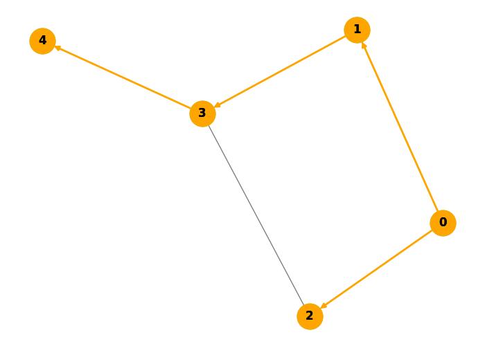
Step-by-Step BFS Traversal:

Start at Node 0 (Source):

• Add Node 0 to the queue.
• Queue: [0]
• Visited: {0}

Explore Node 0:

• The neighbors of Node 0 are Node 1 and Node 2.
• Add Node 1 and Node 2 to the queue.
• Queue: [1, 2]
• Visited: {0, 1, 2}

Explore Node 1:

• The neighbors of Node 1 are Node 0 (already visited) and Node 3.
• Add Node 3 to the queue.
• Queue: [2, 3]
• Visited: {0, 1, 2, 3}

Explore Node 2:

• The neighbors of Node 2 are Node 0 (already visited) and Node 3 (already visited).
• No new nodes are added to the queue.
• Queue: [3]
• Visited: {0, 1, 2, 3}

Explore Node 3:

• The neighbors of Node 3 are Node 1 (already visited) and Node 4.
• Add Node 4 to the queue.
• Queue: [4]
• Visited: {0, 1, 2, 3, 4}

Explore Node 4:

• The neighbors of Node 4 are Node 3 (already visited).
• No new nodes are added to the queue.
• Queue: [] (empty)

At this point, the queue is empty, and all reachable nodes have been visited. The traversal order is: 0, 1, 2, 3, 4

Depth-First Search (DFS)

The Depth-First Search (DFS) algorithm explores as deeply as possible into the graph, visiting one neighbor of each node before moving to the next unvisited neighbor. If no unvisited neighbors are found, it backtracks to the previous node.

The DFS traversal begins at the source node (Node 0) and explores each branch before backtracking.

• Adjacency List: O(V + E)
• Adjacency Matrix: O(V²)

Similar to BFS, the time complexity of DFS is O(V + E) for adjacency lists, as it explores every vertex and edge once.

In the following image, the edges in the DFS traversal path are colored red −

Step-by-Step Depth-First Search (DFS) Traversal:

Start at Node 0 (Source):

• Push Node 0 onto the stack.
• Stack: [0]
• Visited: {0}

Explore Node 0:

• The neighbors of Node 0 are Node 1 and Node 2.
• DFS follows the first neighbor, so it goes to Node 1.
• Push Node 1 onto the stack.
• Stack: [0, 1]
• Visited: {0, 1}

Explore Node 1:

• The neighbors of Node 1 are Node 0 (already visited) and Node 3.
• DFS moves to Node 3 as it hasn't been visited yet.
• Push Node 3 onto the stack.
• Stack: [0, 1, 3]
• Visited: {0, 1, 3}

Explore Node 3:

• The neighbors of Node 3 are Node 1 (already visited) and Node 4.
• DFS moves to Node 4 as it hasn't been visited yet.
• Push Node 4 onto the stack.
• Stack: [0, 1, 3, 4]
• Visited: {0, 1, 3, 4}

Explore Node 4:

• The neighbors of Node 4 are Node 3 (already visited).
• No new nodes to visit, so backtrack to Node 3.
• Stack: [0, 1, 3]
• Visited: {0, 1, 3, 4}

Backtrack to Node 3:

• Since all neighbors of Node 3 have been visited, backtrack to Node 1.
• Stack: [0, 1]
• Visited: {0, 1, 3, 4}

Backtrack to Node 1:

• All neighbors of Node 1 have been visited, so backtrack to Node 0.
• Stack: [0]
• Visited: {0, 1, 3, 4}

Explore Node 2:

• The neighbor of Node 2 is Node 0 (already visited).
• No new nodes to visit, and the stack is now empty.

End of DFS Traversal:

• All reachable nodes from Node 0 have been visited.
• The traversal order is: 0, 1, 3, 4, 2

Dijkstra's Algorithm

Dijkstra's algorithm is used to find the shortest path from a source vertex to all other vertices in a weighted graph. It is commonly used in networking, transportation, and routing algorithms.

The algorithm works by maintaining a set of vertices whose shortest distance from the source is known. It repeatedly selects the vertex with the smallest known distance, explores its neighbors, and updates their distances. It uses a priority queue to achieve efficiency.

• Using a Priority Queue: O((V + E) log V)
• Without a Priority Queue: O(V²)

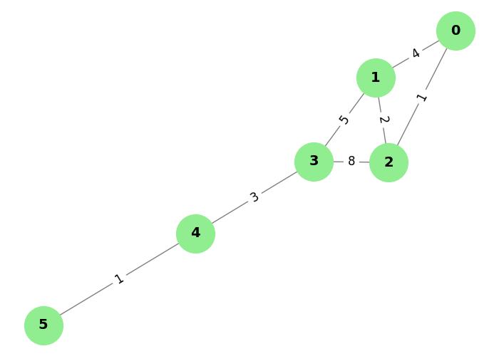
In the above image,

Shortest distances from source node 0:
Node 0: 0
Node 1: 3
Node 2: 1
Node 3: 8
Node 4: 11
Node 5: 12

Shortest path tree (previous nodes):
Node 0: Previous node None
Node 1: Previous node 2
Node 2: Previous node 0
Node 3: Previous node 1
Node 4: Previous node 3
Node 5: Previous node 4

Analysis of Graph Representations

The way we represent a graph affects how fast algorithms can work on it −

• Adjacency List: This method is useful for graphs with fewer edges (sparse graphs). Algorithms that traverse these graphs usually take O(V + E) time, where V is the number of nodes and E is the number of edges.
• Adjacency Matrix: This method works better for graphs with many edges (dense graphs), but algorithms can take O(V²) time to process them, which can be slower for larger graphs.