- Graph Theory - Home
- Graph Theory - Introduction
- Graph Theory - History
- Graph Theory - Fundamentals
- Graph Theory - Applications
- Types of Graphs
- Graph Theory - Types of Graphs
- Graph Theory - Simple Graphs
- Graph Theory - Multi-graphs
- Graph Theory - Directed Graphs
- Graph Theory - Weighted Graphs
- Graph Theory - Bipartite Graphs
- Graph Theory - Complete Graphs
- Graph Theory - Subgraphs
- Graph Theory - Trees
- Graph Theory - Forests
- Graph Theory - Planar Graphs
- Graph Theory - Hypergraphs
- Graph Theory - Infinite Graphs
- Graph Theory - Random Graphs
- Graph Representation
- Graph Theory - Graph Representation
- Graph Theory - Adjacency Matrix
- Graph Theory - Adjacency List
- Graph Theory - Incidence Matrix
- Graph Theory - Edge List
- Graph Theory - Compact Representation
- Graph Theory - Incidence Structure
- Graph Theory - Matrix-Tree Theorem
- Graph Properties
- Graph Theory - Basic Properties
- Graph Theory - Coverings
- Graph Theory - Matchings
- Graph Theory - Independent Sets
- Graph Theory - Traversability
- Graph Theory Connectivity
- Graph Theory - Connectivity
- Graph Theory - Vertex Connectivity
- Graph Theory - Edge Connectivity
- Graph Theory - k-Connected Graphs
- Graph Theory - 2-Vertex-Connected Graphs
- Graph Theory - 2-Edge-Connected Graphs
- Graph Theory - Strongly Connected Graphs
- Graph Theory - Weakly Connected Graphs
- Graph Theory - Connectivity in Planar Graphs
- Graph Theory - Connectivity in Dynamic Graphs
- Special Graphs
- Graph Theory - Regular Graphs
- Graph Theory - Complete Bipartite Graphs
- Graph Theory - Chordal Graphs
- Graph Theory - Line Graphs
- Graph Theory - Complement Graphs
- Graph Theory - Graph Products
- Graph Theory - Petersen Graph
- Graph Theory - Cayley Graphs
- Graph Theory - De Bruijn Graphs
- Graph Algorithms
- Graph Theory - Graph Algorithms
- Graph Theory - Breadth-First Search
- Graph Theory - Depth-First Search (DFS)
- Graph Theory - Dijkstra's Algorithm
- Graph Theory - Bellman-Ford Algorithm
- Graph Theory - Floyd-Warshall Algorithm
- Graph Theory - Johnson's Algorithm
- Graph Theory - A* Search Algorithm
- Graph Theory - Kruskal's Algorithm
- Graph Theory - Prim's Algorithm
- Graph Theory - Borůvka's Algorithm
- Graph Theory - Ford-Fulkerson Algorithm
- Graph Theory - Edmonds-Karp Algorithm
- Graph Theory - Push-Relabel Algorithm
- Graph Theory - Dinic's Algorithm
- Graph Theory - Hopcroft-Karp Algorithm
- Graph Theory - Tarjan's Algorithm
- Graph Theory - Kosaraju's Algorithm
- Graph Theory - Karger's Algorithm
- Graph Coloring
- Graph Theory - Coloring
- Graph Theory - Edge Coloring
- Graph Theory - Total Coloring
- Graph Theory - Greedy Coloring
- Graph Theory - Four Color Theorem
- Graph Theory - Coloring Bipartite Graphs
- Graph Theory - List Coloring
- Advanced Topics of Graph Theory
- Graph Theory - Chromatic Number
- Graph Theory - Chromatic Polynomial
- Graph Theory - Graph Labeling
- Graph Theory - Planarity & Kuratowski's Theorem
- Graph Theory - Planarity Testing Algorithms
- Graph Theory - Graph Embedding
- Graph Theory - Graph Minors
- Graph Theory - Isomorphism
- Spectral Graph Theory
- Graph Theory - Graph Laplacians
- Graph Theory - Cheeger's Inequality
- Graph Theory - Graph Clustering
- Graph Theory - Graph Partitioning
- Graph Theory - Tree Decomposition
- Graph Theory - Treewidth
- Graph Theory - Branchwidth
- Graph Theory - Graph Drawings
- Graph Theory - Force-Directed Methods
- Graph Theory - Layered Graph Drawing
- Graph Theory - Orthogonal Graph Drawing
- Graph Theory - Examples
- Computational Complexity of Graph
- Graph Theory - Time Complexity
- Graph Theory - Space Complexity
- Graph Theory - NP-Complete Problems
- Graph Theory - Approximation Algorithms
- Graph Theory - Parallel & Distributed Algorithms
- Graph Theory - Algorithm Optimization
- Graphs in Computer Science
- Graph Theory - Data Structures for Graphs
- Graph Theory - Graph Implementations
- Graph Theory - Graph Databases
- Graph Theory - Query Languages
- Graph Algorithms in Machine Learning
- Graph Neural Networks
- Graph Theory - Link Prediction
- Graph-Based Clustering
- Graph Theory - PageRank Algorithm
- Graph Theory - HITS Algorithm
- Graph Theory - Social Network Analysis
- Graph Theory - Centrality Measures
- Graph Theory - Community Detection
- Graph Theory - Influence Maximization
- Graph Theory - Graph Compression
- Graph Theory Real-World Applications
- Graph Theory - Network Routing
- Graph Theory - Traffic Flow
- Graph Theory - Web Crawling Data Structures
- Graph Theory - Computer Vision
- Graph Theory - Recommendation Systems
- Graph Theory - Biological Networks
- Graph Theory - Social Networks
- Graph Theory - Smart Grids
- Graph Theory - Telecommunications
- Graph Theory - Knowledge Graphs
- Graph Theory - Game Theory
- Graph Theory - Urban Planning
- Graph Theory Useful Resources
- Graph Theory - Quick Guide
- Graph Theory - Useful Resources
- Graph Theory - Discussion
Graph Theory - Floyd-Warshall Algorithm
Floyd-Warshall Algorithm
The Floyd-Warshall algorithm is used to find the shortest paths between all pairs of vertices in a weighted graph.
It works for both directed and undirected graphs and can handle graphs with negative weights, but it does not work with graphs containing negative weight cycles.
Floyd-Warshall Algorithm Overview
The Floyd-Warshall algorithm calculates the shortest paths between all pairs of vertices in a graph by iteratively updating the shortest paths between every pair of nodes. It relies on dynamic programming and systematically explores each intermediate vertex to check if it provides a shorter path between two nodes.
The algorithm is based on the principle of relaxation, where it iteratively improves the shortest path estimates between nodes by considering intermediate vertices. Initially, it assumes that the shortest path between two vertices is the direct edge between them, and it updates this assumption by checking if a path through an intermediate vertex is shorter.
Steps of the Floyd-Warshall Algorithm
The algorithm proceeds in the following steps −
- Initialize a distance matrix where dist[i][j] is the weight of the direct edge from vertex i to vertex j, or infinity if no edge exists.
- Iterate through each vertex k as an intermediate vertex, and for each pair of vertices (i, j), check if the path from i to j through k is shorter than the direct path. If it is, update dist[i][j] with the shorter path length.
- Repeat the process for all vertices k, i, and j to update the shortest path distances between every pair of vertices.
- After the algorithm terminates, the distance matrix will contain the shortest path lengths between every pair of vertices.
Example of Floyd-Warshall Algorithm
Consider the following weighted graph −
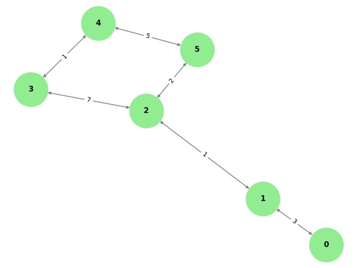
The graph can be represented as the following adjacency matrix, where the value at dist[i][j] represents the weight of the edge from vertex i to vertex j −
dist = [
   [0, 3, inf, inf, inf, inf],
   [3, 0, 1, inf, inf, inf],
   [inf, 1, 0, 7, inf, 2],
   [inf, inf, 7, 0, 1, inf],
   [inf, inf, inf, 1, 0, 5],
   [inf, inf, 2, inf, 5, 0]
]
Here, dist[0][1] = 3 means there is an edge from vertex 0 to vertex 1 with weight 3, and dist[0][2] = inf means there is no direct edge between vertex 0 and vertex 2.
Step 1: Initialization
We initialize the distance matrix with the direct edges between vertices:
dist = [
   [0, 3, inf, inf, inf, inf],
   [3, 0, 1, inf, inf, inf],
   [inf, 1, 0, 7, inf, 2],
   [inf, inf, 7, 0, 1, inf],
   [inf, inf, inf, 1, 0, 5],
   [inf, inf, 2, inf, 5, 0]
]
Step 2: Iteration with k = 0
We now check if any shorter paths can be found through vertex 0. For each pair of vertices i and j, we check if dist[i][j] > dist[i][0] + dist[0][j]. If true, update dist[i][j] with the shorter path.
For example:
- For dist[1][2], we check if dist[1][2] > dist[1][0] + dist[0][2], or 1 > 3 + inf. No update is made since dist[1][0] + dist[0][2] is infinity.
- For dist[2][4], we check if dist[2][4] > dist[2][0] + dist[0][4], or inf > inf + inf. No update is made.
After this iteration, the matrix remains unchanged for k = 0:
dist = [
   [0, 3, inf, inf, inf, inf],
   [3, 0, 1, inf, inf, inf],
   [inf, 1, 0, 7, inf, 2],
   [inf, inf, 7, 0, 1, inf],
   [inf, inf, inf, 1, 0, 5],
   [inf, inf, 2, inf, 5, 0]
]
Step 3: Iteration with k = 1
Next, we check for shorter paths through vertex 1. For each pair (i, j), we check if dist[i][j] > dist[i][1] + dist[1][j]. If true, update dist[i][j] with the shorter path.
For example:
- For dist[0][2], we check if dist[0][2] > dist[0][1] + dist[1][2], or inf > 3 + 1, which is true. Thus, we update dist[0][2] to 4.
- For dist[3][5], we check if dist[3][5] > dist[3][1] + dist[1][5], or inf > inf + inf. No update is made.
After this iteration, the matrix is updated to:
dist = [
   [0, 3, 4, inf, inf, inf],
   [3, 0, 1, inf, inf, inf],
   [4, 1, 0, 7, inf, 2],
   [inf, inf, 7, 0, 1, inf],
   [inf, inf, inf, 1, 0, 5],
   [inf, inf, 2, inf, 5, 0]
]
Step 4: Further Iterations
The process continues for the remaining intermediate vertices k = 2, k = 3, and so on, progressively refining the distance matrix. After all iterations, the final distance matrix will contain the shortest paths between all pairs of vertices.
Step 1: Initialization
[0, 3, '', '', '', '']
[3, 0, 1, '', '', '']
['', 1, 0, 7, '', 2]
['', '', 7, 0, 1, '']
['', '', '', 1, 0, 5]
['', '', 2, '', 5, 0]

Step 2: Iteration with k = 0
[0, 3, '', '', '', '']
[3, 0, 1, '', '', '']
['', 1, 0, 7, '', 2]
['', '', 7, 0, 1, '']
['', '', '', 1, 0, 5]
['', '', 2, '', 5, 0]

Step 3: Iteration with k = 1
[0, 3, 4, '', '', '']
[3, 0, 1, '', '', '']
[4, 1, 0, 7, '', 2]
['', '', 7, 0, 1, '']
['', '', '', 1, 0, 5]
['', '', 2, '', 5, 0]

Step 3: Iteration with k = 2
[0, 3, 4, 11, '', 6]
[3, 0, 1, 8, '', 3]
[4, 1, 0, 7, '', 2]
[11, 8, 7, 0, 1, 9]
['', '', '', 1, 0, 5]
[6, 3, 2, 9, 5, 0]

Step 4: Iteration with k = 3
[0, 3, 4, 11, 12, 6]
[3, 0, 1, 8, 9, 3]
[4, 1, 0, 7, 8, 2]
[11, 8, 7, 0, 1, 9]
[12, 9, 8, 1, 0, 5]
[6, 3, 2, 9, 5, 0]

Step 5: Iteration with k = 4
[0, 3, 4, 11, 12, 6]
[3, 0, 1, 8, 9, 3]
[4, 1, 0, 7, 8, 2]
[11, 8, 7, 0, 1, 6]
[12, 9, 8, 1, 0, 5]
[6, 3, 2, 6, 5, 0]

Step 6: Iteration with k = 5
[0, 3, 4, 11, 11, 6]
[3, 0, 1, 8, 8, 3]
[4, 1, 0, 7, 7, 2]
[11, 8, 7, 0, 1, 6]
[11, 8, 7, 1, 0, 5]
[6, 3, 2, 6, 5, 0]

Final distance matrix after all iterations
[0, 3, 4, 11, 11, 6]
[3, 0, 1, 8, 8, 3]
[4, 1, 0, 7, 7, 2]
[11, 8, 7, 0, 1, 6]
[11, 8, 7, 1, 0, 5]
[6, 3, 2, 6, 5, 0]
Complexity of Floyd-Warshall Algorithm
The time complexity of the Floyd-Warshall algorithm is O(V3), where V is the number of vertices in the graph. This is because the algorithm uses three nested loops, each iterating over all vertices.
The space complexity is O(V2), as it requires storing the distance matrix with V x V entries to represent the shortest paths between all pairs of vertices.
Applications of Floyd-Warshall Algorithm
The Floyd-Warshall algorithm has various applications, such as −
- All-Pairs Shortest Path: The Floyd-Warshall algorithm is used to find the shortest path between every pair of vertices in a graph.
- Network Analysis: It is used in network analysis to compute the shortest paths between every pair of nodes in a network, helping in routing and optimization.
- Transitive Closure: The algorithm can be used to calculate the transitive closure of a directed graph, helping to determine reachability between nodes.
- Graph Connectivity: It is used to analyze graph connectivity by finding paths between all pairs of vertices.
Floyd-Warshall Algorithm in Python
Following is an implementation of the Floyd-Warshall algorithm in Python −
def floyd_warshall(graph):
   # Initialize the distance matrix
   dist = [[float('inf')] * len(graph) for _ in range(len(graph))]
   for i in range(len(graph)):
      dist[i][i] = 0
   for u in range(len(graph)):
      for v, weight in graph[u]:
         dist[u][v] = weight

   # Perform the Floyd-Warshall algorithm
   for k in range(len(graph)):
      for i in range(len(graph)):
         for j in range(len(graph)):
            if dist[i][j] > dist[i][k] + dist[k][j]:
               dist[i][j] = dist[i][k] + dist[k][j]

   return dist

# Example graph (Adjacency list representation)
graph = [
   [(1, 3), (2, 4)],
   [(0, 3), (2, 1)],
   [(1, 1), (3, 7), (5, 2)],
   [(2, 7), (4, 1)],
   [(3, 1), (5, 5)],
   [(2, 2), (4, 5)]
]

# Executing Floyd-Warshall algorithm
distances = floyd_warshall(graph)
for row in distances:
   print(row)
This implementation computes the shortest paths between every pair of vertices in the graph using the Floyd-Warshall algorithm −
[0, 3, 4, 11, 11, 6]
[3, 0, 1, 8, 8, 3]
[4, 1, 0, 7, 7, 2]
[11, 8, 7, 0, 1, 6]
[11, 8, 7, 1, 0, 5]
[6, 3, 2, 6, 5, 0]
