Graph Theory - Link Prediction

---

---

Link Prediction

Link prediction is a task in graph theory and machine learning where the goal is to predict the existence of a link (or edge) between two nodes in a graph that is not yet present.

It assumes that relationships between nodes evolve over time and that these relationships can be predicted based on existing patterns in the graph.

Why is Link Prediction Important?

Link prediction has practical importance in various fields, such as −

• Social Networks: Suggesting new connections or friendships between users based on existing interactions.
• Recommendation Systems: Predicting which products a user may be interested in by identifying unobserved relationships.
• Bioinformatics: Predicting interactions between proteins or genes in biological networks.
• Knowledge Graphs: Adding missing relationships between entities to enhance the graph's usefulness.

Types of Link Prediction Tasks

Link prediction can be categorized based on the type of prediction being made −

• Binary Link Prediction: Predicting whether a link exists or not between two nodes.
• Top-N Link Prediction: Predicting the top N potential links that might form in the future.

Basic Concepts in Link Prediction

To understand link prediction techniques, it is important to know the fundamental graph-based concepts −

• Node Similarity: Similarity between two nodes in the graph based on their structure and attributes.
• Common Neighbors: Nodes that share common neighbors are more likely to be connected.
• Path Length: Shorter paths between nodes indicates stronger potential links.
• Graph Embeddings: Low-dimensional vector representations of graph nodes that capture structural information.

Approaches to Link Prediction

There are several approaches to link prediction, each based on different assumptions and methodologies −

Similarity-based Methods

These methods are based on the assumption that nodes that are structurally similar are likely to be connected. Common similarity measures are as follows −

• Common Neighbors: The number of common neighbors between two nodes. If two nodes have many common neighbors, they are likely to form a link.
• Jaccard Coefficient: The ratio of common neighbors to the total number of neighbors for two nodes:

Machine Learning-based Methods

These methods use graph features (e.g., node embeddings, degrees, common neighbors) as inputs to machine learning models −

• Supervised Learning: A classifier (e.g., logistic regression, random forest) is trained on a set of positive and negative links.
• Graph Embeddings: Graphs are embedded into low-dimensional spaces using techniques like DeepWalk, Node2Vec, or Graph Convolutional Networks (GCNs). These embeddings capture graph structure and node similarity for link prediction.

Probabilistic Models

Probabilistic models predict link formation by learning from graph structure and node attributes. One common approach is using matrix factorization techniques like Singular Value Decomposition (SVD) or probabilistic matrix factorization, where the goal is to predict missing values in the adjacency matrix of the graph.

Evaluation Metrics for Link Prediction

To assess the performance of link prediction algorithms, several evaluation metrics are commonly used −

• Precision: The proportion of predicted links that are correct.
• Recall: The proportion of actual links that are correctly predicted.
• F1-Score: The harmonic mean of precision and recall.
• AUC-ROC: The area under the receiver operating characteristic curve, which evaluates the ability to distinguish between positive and negative links.

Link Prediction Example Using NetworkX

In this section, we demonstrate a simple link prediction task using NetworkX and Python. We will use the common neighbors similarity method.

• Step 1: Importing Necessary Libraries

import networkx as nx
from itertools import combinations

Step 2: Creating a Graph

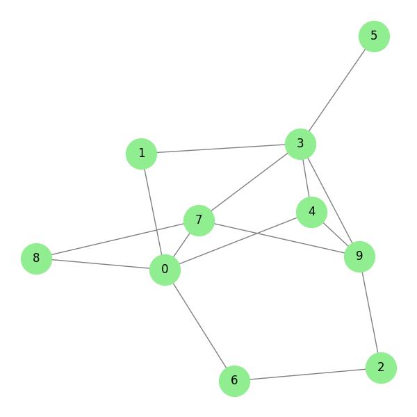
# Create a random graph with 10 nodes and 40% edge probability
G = nx.erdos_renyi_graph(10, 0.4)  
nx.draw(G, with_labels=True)

Step 3: Computing Similarity Based on Common Neighbors

def common_neighbors_score(G, node1, node2):
   common_neighbors = list(nx.common_neighbors(G, node1, node2))
   return len(common_neighbors)

edges = list(combinations(G.nodes, 2))
scores = [(u, v, common_neighbors_score(G, u, v)) for u, v in edges]
scores_sorted = sorted(scores, key=lambda x: x[2], reverse=True)

# Display top predicted links
top_links = scores_sorted[:5]
print(top_links)

Complete Example

Following is the complete Python code combining all steps into a single executable program −

import networkx as nx
import matplotlib.pyplot as plt
from itertools import combinations

# Step 1: Create a random graph with 10 nodes and 40% edge probability
G = nx.erdos_renyi_graph(10, 0.4)

# Draw the graph
plt.figure(figsize=(6, 6))
nx.draw(G, with_labels=True, node_color='lightblue', edge_color='gray', node_size=1000, font_size=12)
plt.title("Generated Random Graph")
plt.show()

# Step 2: Define a function to compute common neighbors similarity
def common_neighbors_score(G, node1, node2):
   common_neighbors = list(nx.common_neighbors(G, node1, node2))
   return len(common_neighbors)

# Step 3: Compute similarity scores for all possible node pairs
edges = list(combinations(G.nodes, 2))
scores = [(u, v, common_neighbors_score(G, u, v)) for u, v in edges]
scores_sorted = sorted(scores, key=lambda x: x[2], reverse=True)

# Step 4: Display top predicted links
top_links = scores_sorted[:5]
print("\nTop 5 Predicted Links Based on Common Neighbors:")
for link in top_links:
   print(f"Nodes {link[0]} - {link[1]} have {link[2]} common neighbors")

The output will show the top 5 predicted links based on common neighbours as shown below −

Top 5 Predicted Links Based on Common Neighbors:
Nodes 0 - 3 have 3 common neighbors
Nodes 4 - 7 have 3 common neighbors
Nodes 0 - 9 have 2 common neighbors
Nodes 1 - 4 have 2 common neighbors
Nodes 1 - 7 have 2 common neighbors

Link Prediction in Real-World Applications

Link prediction is used in various real-world scenarios, such as −

• Social Networks: Predicting new friendships, followers, or interactions.
• Recommendation Systems: Suggesting products, movies, or music to users based on unobserved preferences.
• Biological Networks: Predicting interactions between proteins or genes in biological systems.
• Fraud Detection: Detecting fraudulent activities in financial networks.

Challenges in Link Prediction

Despite its success, link prediction faces several challenges −

• Dynamic Graphs: The structure of the graph may evolve over time, requiring adaptive models.
• Sparse Data: Many real-world graphs are sparse, making it difficult to learn accurate models.
• Scalability: Link prediction on large-scale graphs can be computationally expensive and time-consuming.