Graph Theory - Space Complexity

---

---

Space Complexity

Space complexity in graph theory refers to the amount of memory required by an algorithm to process a graph. It evaluates how the memory usage changes as the graph grows in size, usually based on the number of vertices (V) and edges (E) in the graph.

In this tutorial, we will explore the space complexity of common graph algorithms and understand how the space requirements vary based on the graph representation.

Space Complexity Notation

Space complexity is expressed using the Big-O notation, which describes the maximum amount of memory required by an algorithm relative to the input size. For graph algorithms, the input size is often measured in terms of −

• V: Number of vertices in the graph.
• E: Number of edges in the graph.

The space complexity of graph algorithms depends significantly on the graph's representation and the additional data structures used during algorithm execution, such as queues, stacks, and arrays.

Graph Algorithms Space Complexity

Space complexity varies depending on the algorithm's design and the graph representation. Here, we will analyze the space complexity of common graph algorithms such as BFS, DFS, and Dijkstra's algorithm.

BFS (Breadth-First Search) Traversal

Breadth-First Search (BFS) is an algorithm used to explore all the vertices in a graph. It starts at a source node, explores all the neighbors at the present depth level, before moving on to nodes at the next depth level.

In the given example, the BFS traversal starts from node 0. The algorithm first explores all immediate neighbors (nodes 1 and 2), and then proceeds to their neighbors (nodes 3, 4, and 5), visiting each node once. The traversal order is shown in orange nodes in the graph.

The BFS algorithm ensures that it visits all the nodes level by level, guaranteeing that the shortest path in terms of edges is found in an unweighted graph. It uses a queue data structure to manage the order of exploration, pushing neighboring nodes into the queue and processing them in the order they were added.

For example, in the traversal order −

• Start from node 0, its neighbors are node 1 and node 2.
• Move to node 1 and explore its neighbors, which are node 3 and node 4.
• Next, visit node 2 and explore its neighbor, node 5.
• Finally, visit nodes 3, 4, and 5, ensuring each node is visited once.

The algorithm guarantees that each node is processed in the shortest possible time, and its computational complexity is O(V + E), where V is the number of vertices and E is the number of edges in the graph.

DFS (Depth-First Search) Traversal

Depth-First Search (DFS) is an algorithm used to explore a graph by starting at a source node and exploring as far as possible along each branch before backtracking.

In the DFS example, the algorithm begins at node 0 and explores one branch fully before moving to another branch. The traversal order is shown in orange nodes in the graph, highlighting how the algorithm moves deeper into the graph before backtracking.

In the above given graph image −

• Start from node 0, the algorithm moves to node 1, and from node 1, it goes deeper to node 3.
• After visiting node 3, it backtracks to node 1 and then visits node 4.
• Once node 4 is visited, it backtracks to node 0 and moves on to node 2.
• From node 2, it goes deeper to node 5 and finishes the exploration.

DFS is well-suited for exploring all possible paths and is commonly used for solving problems like finding connected components, topological sorting, and solving puzzles like mazes. The algorithm uses a stack data structure (or recursion) to keep track of nodes to visit.

The DFS algorithm has a time complexity of O(V + E), similar to BFS, where V is the number of vertices and E is the number of edges. The key difference is that DFS explores deep into one branch before backtracking, while BFS explores level by level.

Dijkstra's Algorithm for Shortest Path

Dijkstra's Algorithm is a famous algorithm used to find the shortest path from a source node to all other nodes in a weighted graph. Unlike BFS and DFS, which are used for unweighted graphs, Dijkstra's works with edge weights and guarantees finding the minimum distance.

In the provided example image, Dijkstra's Algorithm begins at node 0, calculating the shortest distance to all other nodes. The graph includes weighted edges, which affect the traversal path. The algorithm keeps track of the shortest known distance to each node and updates it as it finds better paths.

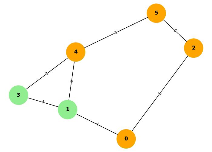
Here, are the traversal steps,

• Start at node 0: with the initial distances to all nodes set to infinity, except the source node, which has a distance of 0.
• Move to node 1: calculating the distance from node 0 (distance = 4). Update the distance of node 1.
• Move to node 2: and update the distance of node 2 to 1.
• From node 2: move to node 5 with a distance of 6.
• Finally, calculate the shortest path to node 4: which is found via node 1 with a total distance of 10.

Step-by-Step Dijkstra's Algorithm Execution:

Step 1: Initialization:

We begin by initializing the distance to all nodes as infinity (), except the starting node (node 0), which has a distance of 0.

Distances: {0: 0, 1: , 2: , 3: , 4: , 5: }
Priority queue: [(0, 0)]  # Start with node 0 and its distance of 0

Step 2: Start at node 0:

We pop the node with the smallest distance (node 0 with distance 0) from the priority queue and explore its neighbors:

• Neighbor node 1: The current distance to node 1 is , but we can reach node 1 from node 0 with a distance of 4. So, we update the distance for node 1 to 4.
• Neighbor node 2: The current distance to node 2 is , but we can reach node 2 from node 0 with a distance of 1. So, we update the distance for node 2 to 1.

Updated Distances: {0: 0, 1: 4, 2: 1, 3: , 4: , 5: }
Priority queue: [(1, 2), (4, 1)]  # Nodes 2 and 1 with updated distances

Step 3: Move to node 2:

Next, we pop node 2 (distance 1) and explore its neighbors:

• Neighbor node 5: The current distance to node 5 is , but we can reach node 5 from node 2 with a distance of 6. So, we update the distance for node 5 to 7.

Updated Distances: {0: 0, 1: 4, 2: 1, 3: , 4: , 5: 7}
Priority queue: [(4, 1), (7, 5)]  # Nodes 1 and 5 with updated distances

Step 4: Move to node 1:

We pop node 1 (distance 4) and explore its neighbors:

• Neighbor node 3: The current distance to node 3 is , but we can reach node 3 from node 1 with a distance of 9. So, we update the distance for node 3 to 9.
• Neighbor node 4: The current distance to node 4 is , but we can reach node 4 from node 1 with a distance of 10. So, we update the distance for node 4 to 10.

Updated Distances: {0: 0, 1: 4, 2: 1, 3: 9, 4: 10, 5: 7}
Priority queue: [(7, 5), (9, 3), (10, 4)]  # Nodes 5, 3, and 4 with updated distances

Step 5: Move to node 5:

We pop node 5 (distance 7) and explore its neighbors:

• No new updates: Since node 5 only connects to node 4, and the current distance to node 4 (10) is smaller than 11, we do not update the distance for node 4.

Distances remain unchanged after processing node 5:
Distances: {0: 0, 1: 4, 2: 1, 3: 9, 4: 10, 5: 7}

Step 6: Move to node 3:

We pop node 3 (distance 9) and explore its neighbors:

• Neighbor node 4: The current distance to node 4 is 10, but we can reach node 4 from node 3 with a distance of 11. Since 11 is greater than the current distance (10), we do not update the distance for node 4.

Distances remain unchanged after processing node 3:
Distances: {0: 0, 1: 4, 2: 1, 3: 9, 4: 10, 5: 7}

Step 7: Move to node 4:

Finally, we pop node 4 (distance 10) and process it. Since it is the last node in the queue, we finish the algorithm here.

Final Distances: {0: 0, 1: 4, 2: 1, 3: 9, 4: 10, 5: 7}

Final Shortest Path Calculation:

The shortest path from node 0 to node 4 is: 0 1 4 with a total distance of 10.

The important detail of Dijkstra's Algorithm is that it processes nodes in the order of their current shortest distance. The priority queue (min-heap) helps in selecting the next node with the smallest known distance. This greedy approach ensures that the shortest path is found efficiently.

The algorithm has a time complexity of O((V + E) log V)) when implemented with a priority queue. Here V is the number of vertices and E is the number of edges, and the logarithmic factor arises due to the priority queue operations.

Analysis of Graph Representations

The space complexity of graph algorithms is significantly impacted by how the graph is represented. Different representations can affect both the algorithm's performance and the space required for the computations.

• Adjacency List: This representation is space-efficient for sparse graphs. The adjacency list requires O(V + E) space, where V is the number of vertices and E is the number of edges.
• Adjacency Matrix: This representation uses O(V²) space, making it less efficient for sparse graphs but better for dense graphs, where the number of edges is close to the maximum possible.

When considering the space complexity of algorithms, it is essential to take into account not only the algorithm's internal data structures (queues, stacks, etc.) but also the underlying graph representation. Depending on whether the graph is dense or sparse, the space complexity can vary significantly.