Graph Theory - Connectivity in Planar Graphs

---

---

Connectivity in Planar Graphs

Connectivity in planar graphs refers to how well the vertices (or nodes) of the graph are linked together by edges (or lines). A planar graph is a type of graph that can be drawn on a flat surface without any of the edges crossing each other.

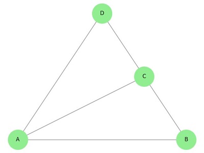
Following image displays a simple planar graph −

Properties of Connectivity in Planar Graphs

Connectivity in planar graphs have various properties, they are −

• Kuratowski's Theorem: A graph is planar if and only if it does not contain a subgraph that is homeomorphic to either K₅ (complete graph on five vertices) or K_3,3 (complete bipartite graph on six vertices).
• Euler's Formula: For a connected planar graph with V vertices, E edges, and F faces, Euler's formula states that V - E + F = 2.
• Edge Bounds: A simple connected planar graph with V vertices has at most 3V - 6 edges.
• Dual Graph: Every planar graph has a corresponding dual graph, where vertices represent faces of the original graph and edges connect vertices of adjacent faces.
• Face Connectivity: The faces in a planar graph are bounded by cycles of edges. The connectivity between these faces can be analyzed using the dual graph.

Homeomorphic is a term used in graph theory to describe a relationship between two graphs. Two graphs are said to be homeomorphic if they can be transformed into each other by a series of simple transformations. These transformations involve either:

• Subdivision of Edges: Adding a new vertex along an edge, effectively breaking the edge into two edges with the new vertex in between.
• Smoothing of Vertices: Removing a vertex of degree two (a vertex connected to exactly two other vertices) and merging its two adjacent edges into a single edge.

Types of Connectivity

Connectivity in planar graphs can be classified into several types −

• Vertex Connectivity: The minimum number of vertices that need to be removed to disconnect the remaining vertices.
• Edge Connectivity: The minimum number of edges that need to be removed to disconnect the graph.
• Path Connectivity: The ability to find paths between pairs of vertices without crossing edges in a planar drawing.
• Face Connectivity: Connectivity between faces in the dual graph, which represents the original graph's faces as vertices.

Vertex Connectivity

Vertex connectivity () of a planar graph is the minimum number of vertices that must be removed to disconnect the graph. It gives details of how strong is the structure of the graph.

• High Connectivity: A highly connected planar graph has a large vertex connectivity value, indicating that more vertices need to be removed to disconnect the graph.
• Low Connectivity: A planar graph with low vertex connectivity can be easily disconnected by removing a few vertices.

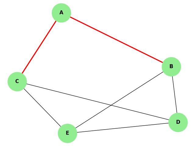
Example

In the following planar graph, removing vertices A and B disconnects the graph, so the vertex connectivity is 2 −

Edge Connectivity

Edge connectivity () of a planar graph is the minimum number of edges that must be removed to disconnect the graph. It measures the strongness of the connectivity of graph against edge removals.

• High Edge Connectivity: A high edge connectivity indicates that the graph remains connected even if several edges are removed.
• Low Edge Connectivity: A graph with low edge connectivity can be easily disconnected by removing a few edges.

Example

In the following planar graph, removing edges (A, B) and (A, C) disconnects the graph, so the edge connectivity is 2 −

Path Connectivity

Path connectivity in a planar graph refers to how easily you can find paths between pairs of vertices without any of the edges crossing each other. It focuses on the ease of traversal within the graph while maintaining its planar properties.

• High Path Connectivity: A graph with high path connectivity allows for multiple non-crossing paths between any two vertices, indicating strong traversal options.
• Low Path Connectivity: A graph with low path connectivity may have limited paths between vertices that do not cross, making traversal more challenging.

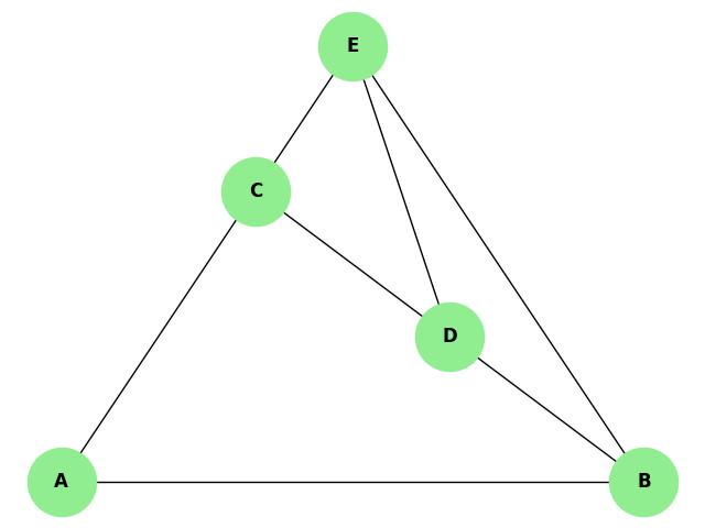
Example

In the following planar graph, paths can be found between any two vertices without crossing edges, demonstrating good path connectivity −

Face Connectivity

Face connectivity in a planar graph refers to how the faces created by the edges of the graph are connected to each other.

Following is the simpler explanation −

• Faces: When you draw a planar graph, it divides the plane into different regions called faces. Each face is an area enclosed by the edges of the graph.
• Dual Graph: To understand face connectivity, we use a concept called the dual graph. In the dual graph, each face of the original graph becomes a vertex.
• Face Connectivity: It looks at how these faces (now vertices in the dual graph) are connected to each other. If the faces are well connected, the graph has good face connectivity.

We have two different types of face connectivity −

• High Face Connectivity: A graph with high face connectivity has strongly connected regions, meaning the faces are well-linked in the dual graph.
• Low Face Connectivity: A graph with low face connectivity has weakly connected regions, indicating that the faces are not as well-linked in the dual graph.

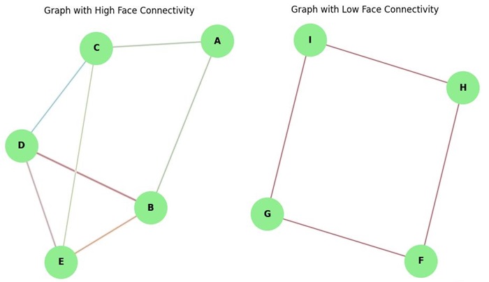
Example

In the following image, a graph is created with edges forming multiple faces that share many common edges, demonstrating high face connectivity. Also, a separate graph is created with edges forming a single face, demonstrating low face connectivity −

Applications of Planar Graphs Connectivity

Connectivity in planar graphs is used in various practical applications, including −

• Network Design: Ensuring strong connectivity in communication and transportation networks, which can be modeled as planar graphs.
• Geographical Mapping: Modeling and analyzing geographical regions and maps, where regions are represented as faces in planar graphs.
• Circuit Layout: Designing circuits where components are laid out on a plane to avoid crossing connections, ensuring connectivity.
• Computer Graphics: Rendering scenes in computer graphics where connectivity between elements must be maintained without overlap.

Testing Connectivity in Planar Graphs

Several algorithms and methods can be used to test connectivity in planar graphs, such as −

• Depth-First Search (DFS): DFS can be used to explore the graph and determine connectivity by checking for paths between all pairs of vertices.
• Breadth-First Search (BFS): Similar to DFS, BFS can be used to test connectivity by exploring the graph level by level.
• Planarity Testing Algorithms: Special algorithms like the Hopcroft-Tarjan planarity test can be used to check if a graph is planar and assess its connectivity.

Special Cases of Planar Graphs

There are several special types of planar graphs that have unique connectivity properties, such as −

Graph Type	Connectivity	Notes
Triangulated Graph	High	Every face is a triangle, leading to high vertex and edge connectivity.
Outerplanar Graph	Moderate	Can be drawn without crossings with all vertices on the outer face.
Grid Graph	Variable	Connectivity depends on the grid's size and structure.
Tree	Low	As a special case of planar graphs, trees have minimal connectivity.
Wheel Graph	High	The central vertex connects to all other vertices, providing high connectivity.
Star Graph	Low	Similar to trees, star graphs have low connectivity.
Hexagonal Graph	Moderate	Common in chemical structure modeling with moderate connectivity.