- Graph Theory - Home
- Graph Theory - Introduction
- Graph Theory - History
- Graph Theory - Fundamentals
- Graph Theory - Applications
- Types of Graphs
- Graph Theory - Types of Graphs
- Graph Theory - Simple Graphs
- Graph Theory - Multi-graphs
- Graph Theory - Directed Graphs
- Graph Theory - Weighted Graphs
- Graph Theory - Bipartite Graphs
- Graph Theory - Complete Graphs
- Graph Theory - Subgraphs
- Graph Theory - Trees
- Graph Theory - Forests
- Graph Theory - Planar Graphs
- Graph Theory - Hypergraphs
- Graph Theory - Infinite Graphs
- Graph Theory - Random Graphs
- Graph Representation
- Graph Theory - Graph Representation
- Graph Theory - Adjacency Matrix
- Graph Theory - Adjacency List
- Graph Theory - Incidence Matrix
- Graph Theory - Edge List
- Graph Theory - Compact Representation
- Graph Theory - Incidence Structure
- Graph Theory - Matrix-Tree Theorem
- Graph Properties
- Graph Theory - Basic Properties
- Graph Theory - Coverings
- Graph Theory - Matchings
- Graph Theory - Independent Sets
- Graph Theory - Traversability
- Graph Theory Connectivity
- Graph Theory - Connectivity
- Graph Theory - Vertex Connectivity
- Graph Theory - Edge Connectivity
- Graph Theory - k-Connected Graphs
- Graph Theory - 2-Vertex-Connected Graphs
- Graph Theory - 2-Edge-Connected Graphs
- Graph Theory - Strongly Connected Graphs
- Graph Theory - Weakly Connected Graphs
- Graph Theory - Connectivity in Planar Graphs
- Graph Theory - Connectivity in Dynamic Graphs
- Special Graphs
- Graph Theory - Regular Graphs
- Graph Theory - Complete Bipartite Graphs
- Graph Theory - Chordal Graphs
- Graph Theory - Line Graphs
- Graph Theory - Complement Graphs
- Graph Theory - Graph Products
- Graph Theory - Petersen Graph
- Graph Theory - Cayley Graphs
- Graph Theory - De Bruijn Graphs
- Graph Algorithms
- Graph Theory - Graph Algorithms
- Graph Theory - Breadth-First Search
- Graph Theory - Depth-First Search (DFS)
- Graph Theory - Dijkstra's Algorithm
- Graph Theory - Bellman-Ford Algorithm
- Graph Theory - Floyd-Warshall Algorithm
- Graph Theory - Johnson's Algorithm
- Graph Theory - A* Search Algorithm
- Graph Theory - Kruskal's Algorithm
- Graph Theory - Prim's Algorithm
- Graph Theory - Borůvka's Algorithm
- Graph Theory - Ford-Fulkerson Algorithm
- Graph Theory - Edmonds-Karp Algorithm
- Graph Theory - Push-Relabel Algorithm
- Graph Theory - Dinic's Algorithm
- Graph Theory - Hopcroft-Karp Algorithm
- Graph Theory - Tarjan's Algorithm
- Graph Theory - Kosaraju's Algorithm
- Graph Theory - Karger's Algorithm
- Graph Coloring
- Graph Theory - Coloring
- Graph Theory - Edge Coloring
- Graph Theory - Total Coloring
- Graph Theory - Greedy Coloring
- Graph Theory - Four Color Theorem
- Graph Theory - Coloring Bipartite Graphs
- Graph Theory - List Coloring
- Advanced Topics of Graph Theory
- Graph Theory - Chromatic Number
- Graph Theory - Chromatic Polynomial
- Graph Theory - Graph Labeling
- Graph Theory - Planarity & Kuratowski's Theorem
- Graph Theory - Planarity Testing Algorithms
- Graph Theory - Graph Embedding
- Graph Theory - Graph Minors
- Graph Theory - Isomorphism
- Spectral Graph Theory
- Graph Theory - Graph Laplacians
- Graph Theory - Cheeger's Inequality
- Graph Theory - Graph Clustering
- Graph Theory - Graph Partitioning
- Graph Theory - Tree Decomposition
- Graph Theory - Treewidth
- Graph Theory - Branchwidth
- Graph Theory - Graph Drawings
- Graph Theory - Force-Directed Methods
- Graph Theory - Layered Graph Drawing
- Graph Theory - Orthogonal Graph Drawing
- Graph Theory - Examples
- Computational Complexity of Graph
- Graph Theory - Time Complexity
- Graph Theory - Space Complexity
- Graph Theory - NP-Complete Problems
- Graph Theory - Approximation Algorithms
- Graph Theory - Parallel & Distributed Algorithms
- Graph Theory - Algorithm Optimization
- Graphs in Computer Science
- Graph Theory - Data Structures for Graphs
- Graph Theory - Graph Implementations
- Graph Theory - Graph Databases
- Graph Theory - Query Languages
- Graph Algorithms in Machine Learning
- Graph Neural Networks
- Graph Theory - Link Prediction
- Graph-Based Clustering
- Graph Theory - PageRank Algorithm
- Graph Theory - HITS Algorithm
- Graph Theory - Social Network Analysis
- Graph Theory - Centrality Measures
- Graph Theory - Community Detection
- Graph Theory - Influence Maximization
- Graph Theory - Graph Compression
- Graph Theory Real-World Applications
- Graph Theory - Network Routing
- Graph Theory - Traffic Flow
- Graph Theory - Web Crawling Data Structures
- Graph Theory - Computer Vision
- Graph Theory - Recommendation Systems
- Graph Theory - Biological Networks
- Graph Theory - Social Networks
- Graph Theory - Smart Grids
- Graph Theory - Telecommunications
- Graph Theory - Knowledge Graphs
- Graph Theory - Game Theory
- Graph Theory - Urban Planning
- Graph Theory Useful Resources
- Graph Theory - Quick Guide
- Graph Theory - Useful Resources
- Graph Theory - Discussion
Graph Theory - Borvka's Algorithm
Borvka's Algorithm
Borvka's algorithm is a parallelized method for finding the minimum spanning tree (MST) of a graph. It is a greedy algorithm that finds the MST by repeatedly identifying and adding the minimum weight edge from each connected component of the graph until only one connected component remains.
Unlike Prim's and Kruskal's algorithms, Borvka's algorithm works in multiple phases, where in each phase, edges are added in parallel from each component to form the minimum spanning tree.
In a parallelized method, multiple tasks are performed simultaneously, rather than sequentially. In the context of Borvka's algorithm, the term "parallelized" means that the algorithm can process multiple edges from different connected components at the same time.
Overview of Borvka's Algorithm
The main idea behind Borvka's algorithm is to find the minimum weight edge in each connected component of the graph and add these edges to the MST. The process repeats until all vertices are connected into one component, resulting in the minimum spanning tree. The steps involved are as follows:
- Initialization: Start with each vertex as a separate component, and create a set of edges to connect the components.
- Parallel Edge Selection: For each component, select the minimum weight edge that connects the component to another component.
- Edge Addition: Add the selected edges to the MST and merge the components that are connected by the chosen edges.
- Repeat: Repeat the process of edge selection and component merging until there is only one component remaining, which forms the minimum spanning tree.
Properties of Borvka's Algorithm
Borvka's algorithm has several properties that distinguish it from other MST algorithms:
- Greedy Algorithm: Like Prim's and Kruskal's algorithms, Borvka's algorithm is greedy, as it selects the minimum weight edge at each step.
- Parallelism: The algorithm is highly parallelizable, making it efficient for large graphs and distributed computing environments.
- Works for Connected Graphs: Borvka's algorithm is designed for connected graphs, but it can be adapted for disconnected graphs by finding the MST for each component.
- Optimal: Borvka's algorithm guarantees finding the minimum spanning tree, as it always selects the minimum weight edge for each component.
Steps of Borvka's Algorithm
Let us break down the steps of Borvka's algorithm for a better understanding −
- Step 1: Initialization: Start with each vertex as a separate component. Each component will initially have no edges in the MST.
- Step 2: Parallel Edge Selection: In each iteration, for each component, find the minimum weight edge that connects it to any other component.
- Step 3: Edge Addition: Once the minimum edges are selected for each component, add them to the MST and merge the components that are connected by these edges.
- Step 4: Repeat: Repeat the process until only one component remains, which is the minimum spanning tree of the graph.
Example of Borvka's Algorithm
Consider the following graph representation −
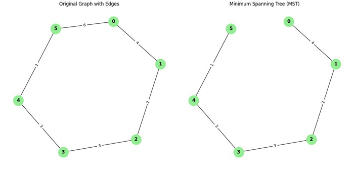
We want to find the minimum spanning tree of the graph using Borvka's algorithm.
Step 1: Initialization
Initially, each vertex is considered its own component. The components are:
components = [{0}, {1}, {2}, {3}, {4}, {5}]
Step 2: Parallel Edge Selection
In the first iteration, we select the minimum edge for each component:
- Component {0}: The minimum edge is (0, 1, 4).
- Component {1}: The minimum edge is (1, 2, 2).
- Component {2}: The minimum edge is (2, 3, 3).
- Component {3}: The minimum edge is (3, 4, 3).
- Component {4}: The minimum edge is (4, 5, 2).
- Component {5}: The minimum edge is (5, 0, 6).
Step 3: Edge Addition
The edges selected in the previous step are added to the MST. After adding these edges, we merge the components:
mst_edges = [(0, 1, 4), (1, 2, 2), (2, 3, 3), (3, 4, 3), (4, 5, 2)]
components = [{0, 1}, {2}, {3, 4, 5}]
Step 4: Repeat
In the second iteration, we repeat the process of selecting the minimum edge for each remaining component:
- Component {0, 1}: The minimum edge is (1, 2, 2).
- Component {2}: The minimum edge is (2, 3, 3).
- Component {3, 4, 5}: The minimum edge is (3, 5, 3).
Step 5: Edge Addition
The edges selected in the second iteration are added to the MST, and the components are merged:
mst_edges = [(0, 1, 4), (1, 2, 2), (2, 3, 3), (3, 4, 3), (4, 5, 2)]
components = [{0, 1, 2, 3, 4, 5}]
At this point, all the components are merged, and we have found the minimum spanning tree.
Complete Python Implementation
Following is the complete Python implementation of Borvka's algorithm −
class Boruvka:
   def __init__(self, num_vertices, edges):
      # Initialize the number of vertices and the list of edges
      self.num_vertices = num_vertices
      self.edges = edges

   def find(self, parent, i):
      # Find the representative (or root) of the component that vertex i belongs to
      if parent[i] == i:
         return i
      else:
         return self.find(parent, parent[i])

   def union(self, parent, rank, x, y):
      # Union of two components: connect the two sets if they are not already connected
      xroot = self.find(parent, x)
      yroot = self.find(parent, y)

      # Union by rank: attach the smaller tree under the larger tree
      if rank[xroot] < rank[yroot]:
         parent[xroot] = yroot
      elif rank[xroot] > rank[yroot]:
         parent[yroot] = xroot
      else:
         parent[yroot] = xroot
         rank[xroot] += 1

   def boruvka_mst(self):
      # Initialize the parent and rank arrays for each vertex
	  # Each vertex is its own parent initially
      parent = [i for i in range(self.num_vertices)]
	  # All components have rank 0 initially
      rank = [0] * self.num_vertices
	  # List to store the edges of the minimum spanning tree
      mst_edges = []
	  # Initially, each vertex is its own component
      num_components = self.num_vertices

      # Continue until there is only one component (the MST is found)
      while num_components > 1:
         # Array to store the cheapest edge for each component
         cheapest = [-1] * self.num_vertices

         # Iterate over all edges and find the cheapest edge for each component
         for u, v, weight in self.edges:
            # Find the components (sets) to which vertices u and v belong
            set_u = self.find(parent, u)
            set_v = self.find(parent, v)

            # If the vertices are in different components, check if this edge is the cheapest for either component
            if set_u != set_v:
               # Update the cheapest edge for the component if this edge has smaller weight
               if cheapest[set_u] == -1 or cheapest[set_u][2] > weight:
                  cheapest[set_u] = (u, v, weight)
               if cheapest[set_v] == -1 or cheapest[set_v][2] > weight:
                  cheapest[set_v] = (u, v, weight)

         # Add the cheapest edges to the MST and update the components
         for i in range(self.num_vertices):
            if cheapest[i] != -1:
               u, v, weight = cheapest[i]
               set_u = self.find(parent, u)
               set_v = self.find(parent, v)

               # If the edge connects two different components, add it to the MST and merge the components
               if set_u != set_v:
			      # Add the edge to the MST
                  mst_edges.append((u, v, weight))
			      # Merge the components
                  self.union(parent, rank, set_u, set_v)
			      # Decrease the number of components
                  num_components -= 1

         # Reset the cheapest array for the next iteration
         cheapest = [-1] * self.num_vertices

      # Return the edges of the minimum spanning tree
      return mst_edges

# Graph represented as a list of edges (u, v, weight)
edges = [
    (0, 1, 4),
    (1, 2, 2),
    (2, 3, 3),
    (3, 4, 3),
    (4, 5, 2),
    (5, 0, 6)
]

# Number of vertices in the graph
num_vertices = 6

# Create an instance of Boruvka's algorithm with the graph's vertices and edges
boruvka = Boruvka(num_vertices, edges)

# Run Borvka's algorithm to find the Minimum Spanning Tree (MST)
mst = boruvka.boruvka_mst()

# Output the MST
print("Minimum Spanning Tree:", mst)
Following is the output obtained −
Minimum Spanning Tree: [(0, 1, 4), (1, 2, 2), (2, 3, 3), (4, 5, 2), (3, 4, 3)]
Complexity Analysis
The time complexity of Borvka's algorithm is O(E log V), where E is the number of edges and V is the number of vertices. This is because, in each iteration, the algorithm processes all edges, and the number of iterations is proportional to the logarithm of the number of vertices.
The space complexity is O(V + E) due to the storage required for components and edges.
Applications of Borvka's Algorithm
Borvka's algorithm is used in various fields where finding a spanning tree is important, such as −
- Parallel Computing: The algorithm is ideal for parallel computing due as it processes multiple edges in each iteration.
- Distributed Systems: Borvka's algorithm is used in distributed systems for network design, where multiple nodes work concurrently to find the minimum spanning tree.
- Telecommunications: Used in designing communication networks.
- Geospatial Applications: Applied in geospatial data analysis for finding optimal routing and connection paths.
