Graph Theory - Graph Laplacian

Quiz

Graph Laplacian

Graph Laplacian is used to study the structure and properties of graphs. It provides information about various aspects of a graph, such as connectivity, diffusion processes, and spectral properties.

The Graph Laplacian of a graph G = (V, E) is a matrix that contains information about the graph's structure, specifically its vertices and edges. It is defined as −

L = D - A

Where,

L is the Laplacian matrix.
D is the degree matrix, a diagonal matrix where each diagonal entry D(i, i) represents the degree (number of edges) of vertex i.
A is the adjacency matrix, where each entry A(i, j) indicates whether there is an edge between vertices i and j.

Example: Laplacian Matrix Calculation

Consider a simple graph with 3 vertices connected in a cycle (a triangle). The adjacency matrix and degree matrix are −

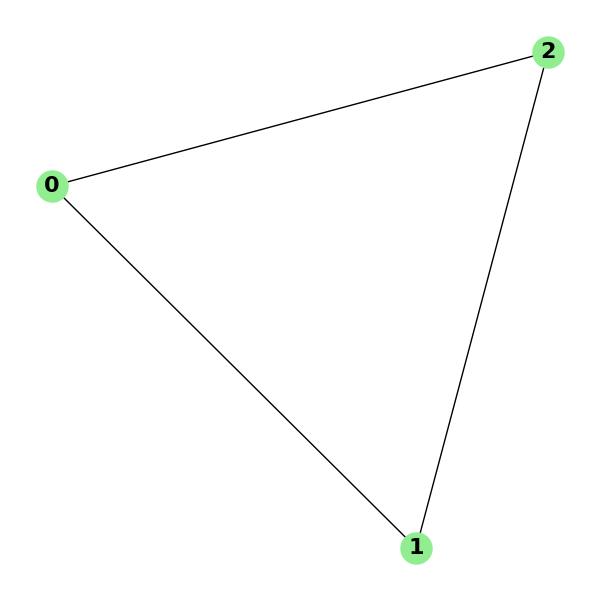
Adjacency matrix A:
[[0, 1, 1],
 [1, 0, 1],
 [1, 1, 0]]

Degree matrix D:
[[2, 0, 0],
 [0, 2, 0],
 [0, 0, 2]]

Laplacian matrix L:
[[ 2, -1, -1],
 [-1,  2, -1],
 [-1, -1,  2]]

The Laplacian matrix of this graph is a symmetric matrix that represents the graph's structure in a concise form. Each row and column corresponds to a vertex, and the matrix encodes information about how the vertices are connected.

Properties of the Graph Laplacian

The Graph Laplacian has several important properties, they are −

Symmetry: The Laplacian matrix is symmetric if the graph is undirected, meaning L = L^T.
Eigenvalues: The eigenvalues of the Laplacian matrix reveal important structural properties of the graph. The smallest eigenvalue is always 0, and its multiplicity indicates the number of connected components in the graph.
Diagonal Entries: The diagonal entries of the Laplacian matrix correspond to the degree of each vertex. This provides information about the local connectivity of vertices.
Sparsity: The Laplacian matrix is generally sparse, especially for large graphs, since most graphs have relatively few edges compared to the number of possible edges.

Example: Eigenvalues of the Laplacian Matrix

Consider the same graph from the previous example (the cycle graph with 3 vertices). The Laplacian matrix was −

Laplacian matrix L:
[[ 2, -1, -1],
 [-1,  2, -1],
 [-1, -1,  2]]

Eigenvalues of the Laplacian matrix: [0, 4, 4]

In this case, the eigenvalues 0, 4, and 4 provide important information about the graph's connectivity and structure. The multiplicity of the eigenvalue 0 indicates that the graph is connected, and the other eigenvalues give details of the graph's overall connectivity and behavior.

Applications of the Graph Laplacian

The Graph Laplacian is used in various applications, such as −

Graph Connectivity: The multiplicity of the eigenvalue 0 of the Laplacian matrix indicates the number of connected components in a graph. A graph is connected if and only if the eigenvalue 0 has multiplicity 1.
Spectral Clustering: Spectral clustering algorithms use the Laplacian matrix to partition a graph into clusters based on the eigenvectors corresponding to the smallest eigenvalues. This technique is commonly used in machine learning for community detection and data segmentation.
Diffusion Processes: The Laplacian matrix is used to model diffusion processes, such as heat diffusion or random walks, on graphs. The eigenvalues and eigenvectors determine how quickly diffusion spreads through the network.
Graph Laplacian Regularization: In machine learning, the Laplacian matrix is commonly used for regularization in graph-based semi-supervised learning, where the goal is to predict labels for nodes in a graph using a combination of labeled and unlabeled data.

Example: Spectral Clustering

Consider a graph with several nodes and edges. The goal is to cluster the nodes into two groups. One way to do this is to use the eigenvectors corresponding to the smallest eigenvalues of the Laplacian matrix. These eigenvectors can be used as features to cluster the nodes into groups that are closely connected.

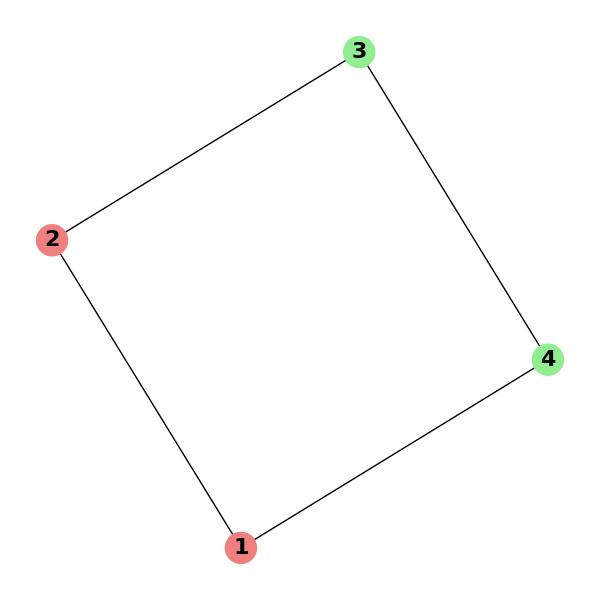
Laplacian matrix L:
[[ 4, -1,  0, -1],
 [-1,  4, -1,  0],
 [ 0, -1,  4, -1],
 [-1,  0, -1,  4]]

Eigenvectors corresponding to the smallest eigenvalues:
[[ 0.5, -0.5],
 [ 0.5,  0.5],
 [ 0.5, -0.5],
 [-0.5,  0.5]]

Clustering the nodes based on the eigenvectors:
Group 1: [1, 2], Group 2: [3, 4]

This example shows how spectral clustering works by partitioning the nodes into two groups based on the eigenvectors of the Laplacian matrix.

Normalized Laplacian Matrix

The normalized Laplacian matrix is a variation of the Laplacian matrix that accounts for vertex degrees. It is defined as −

L_norm = D^(-1/2) * L * D^(-1/2)

Where D^(-1/2) is the inverse square root of the degree matrix. The normalized Laplacian matrix is useful in spectral clustering and graph-based signal processing because it accounts for the degree of vertices and makes the analysis more strong to variations in vertex degrees.

Cheeger's Inequality and Graph Laplacians

Cheeger's inequality relates the second-smallest eigenvalue of the Laplacian matrix to the graph's conductance, a measure of its connectivity. Specifically, Cheeger's inequality states that −

h(G)  ₂ / 2  2 * h(G)

Where, h(G) is the conductance of the graph, and ₂ is the second-smallest eigenvalue of the Laplacian matrix. This inequality provides a way to estimate the graph's connectivity based on its spectral properties.

Print Page