Graph Theory - Petersen Graph

Quiz

Petersen Graph

The Petersen graph is one of the most famous and well-studied graphs in the field of graph theory. It is named after the Danish mathematician Julius Petersen, who first described it in 1898. The Petersen graph is known for its unique properties and numerous applications in various fields of mathematics and computer science.

In this tutorial, we will learn the properties, construction, and applications of the Petersen graph.

Properties of the Petersen Graph

The Petersen graph has several properties that make it an interesting subject of study. Following are some of its key properties −

Vertices: The Petersen graph has 10 vertices.
Edges: It has 15 edges.
Degree: Each vertex has a degree of 3, making it a 3-regular graph.
Non-planarity: The Petersen graph is non-planar, meaning it cannot be drawn on a plane without edges crossing.
Symmetry: It is highly symmetric, having a large automorphism group.
Diameter: The diameter of the Petersen graph is 2.
Chromatic Number: The chromatic number of the Petersen graph is 3.
Girth: The girth (length of the shortest cycle) is 5.

Graph Structure

The Petersen graph can be visualized in different ways, but it is often represented as a star polygon structure with additional edges connecting the vertices. One common representation is as follows:

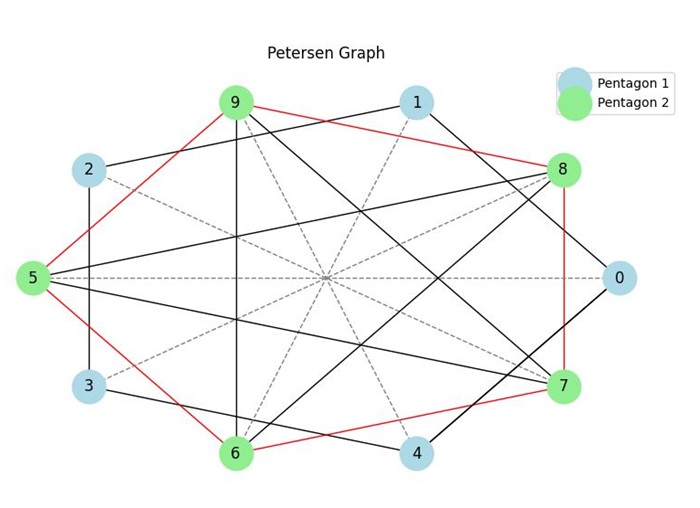
In this representation, the Petersen graph can be seen as a combination of two sets of 5 vertices, each forming a pentagon. The vertices of one pentagon are connected to the vertices of the other pentagon in a particular manner.

Adjacency Matrix

The adjacency matrix of the Petersen graph is a 10x10 matrix that represents the connections between the vertices. Each element A[i][j] is 1 if there is an edge between vertex i and vertex j, and 0 otherwise. Following is the adjacency matrix of the Petersen graph −

0 1 0 0 1 1 0 0 0 0
1 0 1 0 0 0 1 0 0 0
0 1 0 1 0 0 0 1 0 0
0 0 1 0 1 0 0 0 1 0
1 0 0 1 0 0 0 0 0 1
1 0 0 0 0 0 0 1 1 0
0 1 0 0 0 0 1 0 0 1
0 0 1 0 0 1 0 0 1 0
0 0 0 1 0 1 0 1 0 0
0 0 0 0 1 0 1 0 0 1

Construction of the Petersen Graph

The Petersen graph can be constructed in multiple ways, each providing a different perspective on its structure. Here, we will describe two common methods: using the complement of the line graph of K₅ and using a set of pairs.

Complement of the Line Graph of K₅

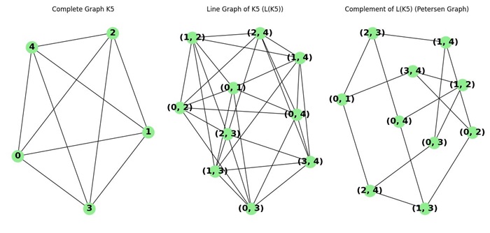
The Petersen graph can be constructed as the complement of the line graph of the complete graph K₅. The steps are as follows −

Start with the complete graph K₅, which has 5 vertices and every pair of vertices is connected by an edge.
Construct the line graph of K₅. The line graph L(K₅) has a vertex for each edge of K₅, and two vertices in L(K₅) are adjacent if and only if their corresponding edges in K₅ share a common vertex.
Take the complement of L(K₅). The complement of a graph G is a graph on the same vertices where two vertices are adjacent if and only if they are not adjacent in G.

The resulting graph is the Petersen graph −

Set of Pairs

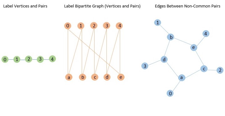
The Petersen graph can also be constructed using a set of pairs. This method involves creating a bipartite graph with two sets of 5 vertices each, where each vertex in one set is connected to exactly two vertices in the other set. The steps are as follows:

Label the vertices as 0, 1, 2, 3, 4 and the pairs as (0,1), (1,2), (2,3), (3,4), (4,0).
Create a bipartite graph with these vertices and pairs, connecting each vertex to the two pairs that include it.
Add edges between pairs that share no common vertex.

The resulting graph is the Petersen graph −

Step-by-Step Explanation

Understanding Pairs: The pairs of vertices are −

(0, 1)
(1, 2)
(2, 3)
(3, 4)
(4, 0)

Determine Common Vertex: For each pair of pair nodes, we need to check whether they share a common vertex from the original vertex set (0, 1, 2, 3, 4). If they do not share any vertex, we add an edge between them −

Let's go through each pair:
Pair 'a' corresponds to (0, 1), which involves vertices 0 and 1.
Pair 'b' corresponds to (1, 2), which involves vertices 1 and 2.
Pair 'c' corresponds to (2, 3), which involves vertices 2 and 3.
Pair 'd' corresponds to (3, 4), which involves vertices 3 and 4.
Pair 'e' corresponds to (4, 0), which involves vertices 4 and 0.

Checking for Common Vertices: Now, we will check each pair of pair nodes to see if they share a vertex:

'a' and 'b': (0, 1) and (1, 2) share vertex 1, so no edge is added.
'a' and 'c': (0, 1) and (2, 3) do not share a vertex, so an edge is added.
'a' and 'd': (0, 1) and (3, 4) do not share a vertex, so an edge is added.
'a' and 'e': (0, 1) and (4, 0) share vertex 0, so no edge is added.
'b' and 'c': (1, 2) and (2, 3) share vertex 2, so no edge is added.
'b' and 'd': (1, 2) and (3, 4) do not share a vertex, so an edge is added.
'b' and 'e': (1, 2) and (4, 0) do not share a vertex, so an edge is added.
'c' and 'd': (2, 3) and (3, 4) share vertex 3, so no edge is added.
'c' and 'e': (2, 3) and (4, 0) do not share a vertex, so an edge is added.
'd' and 'e': (3, 4) and (4, 0) share vertex 4, so no edge is added.

Final Edge List: From the above analysis, we can summarize the pairs that will have edges added between them:

('a', 'c')
('a', 'd')
('b', 'd')
('b', 'e')
('c', 'e')

Coloring of the Petersen Graph

Graph coloring is the assignment of colors to the vertices of a graph such that no two adjacent vertices share the same color. The chromatic number of the Petersen graph is 3, meaning that at least 3 colors are required to color it.

Vertex Coloring

A proper vertex coloring of the Petersen graph using 3 colors can be achieved as follows −

In this coloring, each vertex is assigned one of three colors in such a way that no two adjacent vertices have the same color.

Edge Coloring

Edge coloring assigns colors to the edges of a graph so that no two edges sharing a common vertex have the same color. The edge chromatic number of the Petersen graph is 4, meaning that 4 colors are needed for a proper edge coloring. Here is an example of edge coloring of the Petersen graph:

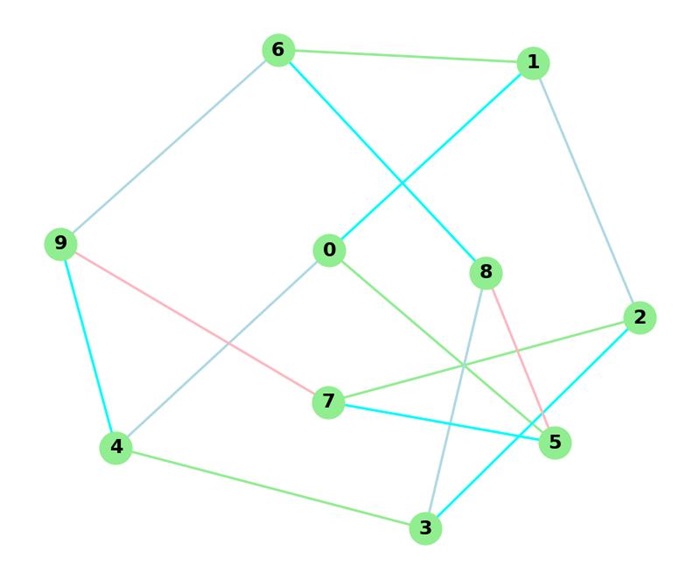
In this edge coloring, each edge is assigned one of four colors such that no two edges sharing a common vertex have the same color.

Automorphisms of the Petersen Graph

An automorphism of a graph is a permutation of its vertices that preserves the adjacency structure. The Petersen graph is known for its high degree of symmetry, having a large automorphism group. The automorphism group of the Petersen graph is isomorphic to the symmetric group S₅, which has 120 elements.

Symmetric Properties

The high degree of symmetry in the Petersen graph means that it looks the same from any vertex or edge, making it vertex-transitive and edge-transitive. This property is significant in various theoretical studies and applications where symmetry plays an important role.

Applications of the Petersen Graph

The Petersen graph has various applications in different areas of mathematics and computer science. Some of the applications are as follows −

Cubic Graphs: The Petersen graph is an important example in the study of cubic graphs, which are graphs where every vertex has a degree of 3.
Graph Theory Problems: It serves as a counterexample in various graph theory problems and conjectures, such as the conjecture that every bridgeless cubic graph contains a Hamiltonian cycle.
Network Design: It's structure is used in the design of certain types of networks and error-correcting codes.
Mathematical Puzzles: The Petersen graph appears in several mathematical puzzles and recreational mathematics problems due to its interesting properties.

Print Page