- Graph Theory - Home
- Graph Theory - Introduction
- Graph Theory - History
- Graph Theory - Fundamentals
- Graph Theory - Applications
- Types of Graphs
- Graph Theory - Types of Graphs
- Graph Theory - Simple Graphs
- Graph Theory - Multi-graphs
- Graph Theory - Directed Graphs
- Graph Theory - Weighted Graphs
- Graph Theory - Bipartite Graphs
- Graph Theory - Complete Graphs
- Graph Theory - Subgraphs
- Graph Theory - Trees
- Graph Theory - Forests
- Graph Theory - Planar Graphs
- Graph Theory - Hypergraphs
- Graph Theory - Infinite Graphs
- Graph Theory - Random Graphs
- Graph Representation
- Graph Theory - Graph Representation
- Graph Theory - Adjacency Matrix
- Graph Theory - Adjacency List
- Graph Theory - Incidence Matrix
- Graph Theory - Edge List
- Graph Theory - Compact Representation
- Graph Theory - Incidence Structure
- Graph Theory - Matrix-Tree Theorem
- Graph Properties
- Graph Theory - Basic Properties
- Graph Theory - Coverings
- Graph Theory - Matchings
- Graph Theory - Independent Sets
- Graph Theory - Traversability
- Graph Theory Connectivity
- Graph Theory - Connectivity
- Graph Theory - Vertex Connectivity
- Graph Theory - Edge Connectivity
- Graph Theory - k-Connected Graphs
- Graph Theory - 2-Vertex-Connected Graphs
- Graph Theory - 2-Edge-Connected Graphs
- Graph Theory - Strongly Connected Graphs
- Graph Theory - Weakly Connected Graphs
- Graph Theory - Connectivity in Planar Graphs
- Graph Theory - Connectivity in Dynamic Graphs
- Special Graphs
- Graph Theory - Regular Graphs
- Graph Theory - Complete Bipartite Graphs
- Graph Theory - Chordal Graphs
- Graph Theory - Line Graphs
- Graph Theory - Complement Graphs
- Graph Theory - Graph Products
- Graph Theory - Petersen Graph
- Graph Theory - Cayley Graphs
- Graph Theory - De Bruijn Graphs
- Graph Algorithms
- Graph Theory - Graph Algorithms
- Graph Theory - Breadth-First Search
- Graph Theory - Depth-First Search (DFS)
- Graph Theory - Dijkstra's Algorithm
- Graph Theory - Bellman-Ford Algorithm
- Graph Theory - Floyd-Warshall Algorithm
- Graph Theory - Johnson's Algorithm
- Graph Theory - A* Search Algorithm
- Graph Theory - Kruskal's Algorithm
- Graph Theory - Prim's Algorithm
- Graph Theory - Borůvka's Algorithm
- Graph Theory - Ford-Fulkerson Algorithm
- Graph Theory - Edmonds-Karp Algorithm
- Graph Theory - Push-Relabel Algorithm
- Graph Theory - Dinic's Algorithm
- Graph Theory - Hopcroft-Karp Algorithm
- Graph Theory - Tarjan's Algorithm
- Graph Theory - Kosaraju's Algorithm
- Graph Theory - Karger's Algorithm
- Graph Coloring
- Graph Theory - Coloring
- Graph Theory - Edge Coloring
- Graph Theory - Total Coloring
- Graph Theory - Greedy Coloring
- Graph Theory - Four Color Theorem
- Graph Theory - Coloring Bipartite Graphs
- Graph Theory - List Coloring
- Advanced Topics of Graph Theory
- Graph Theory - Chromatic Number
- Graph Theory - Chromatic Polynomial
- Graph Theory - Graph Labeling
- Graph Theory - Planarity & Kuratowski's Theorem
- Graph Theory - Planarity Testing Algorithms
- Graph Theory - Graph Embedding
- Graph Theory - Graph Minors
- Graph Theory - Isomorphism
- Spectral Graph Theory
- Graph Theory - Graph Laplacians
- Graph Theory - Cheeger's Inequality
- Graph Theory - Graph Clustering
- Graph Theory - Graph Partitioning
- Graph Theory - Tree Decomposition
- Graph Theory - Treewidth
- Graph Theory - Branchwidth
- Graph Theory - Graph Drawings
- Graph Theory - Force-Directed Methods
- Graph Theory - Layered Graph Drawing
- Graph Theory - Orthogonal Graph Drawing
- Graph Theory - Examples
- Computational Complexity of Graph
- Graph Theory - Time Complexity
- Graph Theory - Space Complexity
- Graph Theory - NP-Complete Problems
- Graph Theory - Approximation Algorithms
- Graph Theory - Parallel & Distributed Algorithms
- Graph Theory - Algorithm Optimization
- Graphs in Computer Science
- Graph Theory - Data Structures for Graphs
- Graph Theory - Graph Implementations
- Graph Theory - Graph Databases
- Graph Theory - Query Languages
- Graph Algorithms in Machine Learning
- Graph Neural Networks
- Graph Theory - Link Prediction
- Graph-Based Clustering
- Graph Theory - PageRank Algorithm
- Graph Theory - HITS Algorithm
- Graph Theory - Social Network Analysis
- Graph Theory - Centrality Measures
- Graph Theory - Community Detection
- Graph Theory - Influence Maximization
- Graph Theory - Graph Compression
- Graph Theory Real-World Applications
- Graph Theory - Network Routing
- Graph Theory - Traffic Flow
- Graph Theory - Web Crawling Data Structures
- Graph Theory - Computer Vision
- Graph Theory - Recommendation Systems
- Graph Theory - Biological Networks
- Graph Theory - Social Networks
- Graph Theory - Smart Grids
- Graph Theory - Telecommunications
- Graph Theory - Knowledge Graphs
- Graph Theory - Game Theory
- Graph Theory - Urban Planning
- Graph Theory Useful Resources
- Graph Theory - Quick Guide
- Graph Theory - Useful Resources
- Graph Theory - Discussion
Graph Theory - Johnson's Algorithm
Johnson's Algorithm
Johnson's algorithm is used for finding the shortest paths between all pairs of vertices in a weighted, directed graph. It is particularly useful for graphs with non-negative weights and is an alternative to the Floyd-Warshall algorithm when the graph has sparse edges.
This algorithm can handle graphs with negative weights, but it requires an additional preprocessing step to detect negative weight cycles, which it cannot handle.
Johnson's algorithm works by performing a series of individual shortest-path calculations from each vertex using a single-source shortest-path algorithm, such as Dijkstra's algorithm. By using reweighting techniques, Johnson's algorithm ensures that all edges have non-negative weights, allowing Dijkstra's algorithm to be used efficiently.
Overview of Johnson's Algorithm
Johnson's algorithm combines two major components −
- Reweighting of edges: A transformation is applied to the graph to eliminate negative weights by assigning a new weight to each edge.
- Shortest-path calculations using Dijkstra's algorithm: After reweighting, Dijkstra's algorithm is used to calculate the shortest paths from each vertex to every other vertex.
While the Floyd-Warshall algorithm has a time complexity of O(V3), Johnson's algorithm has a time complexity of O(V2 log V + VE), where V is the number of vertices and E is the number of edges in the graph. This makes Johnson's algorithm more efficient for sparse graphs with fewer edges.
Steps of Johnson's Algorithm
The Johnson's algorithm proceeds in the following steps −
- Step 1: Add a new vertex: Introduce a new vertex q to the graph and add edges from q to every other vertex with weight 0. This new vertex will be used for the reweighting process.
- Step 2: Apply Bellman-Ford algorithm: Run the Bellman-Ford algorithm from vertex q to calculate the shortest paths from q to all other vertices. This step helps in detecting negative weight cycles.
- Step 3: Reweight edges: Once the shortest path distances from q to every other vertex are known, reweight the edges of the original graph using the formula: weight(u, v) = original weight(u, v) + h(u) - h(v), where h(u) is the shortest path distance from q to vertex u.
- Step 4: Run Dijkstra's algorithm: After reweighting the edges, use Dijkstra's algorithm for each vertex in the graph to compute the shortest paths from each vertex to every other vertex.
- Step 5: Recover the original weights: After executing Dijkstra's algorithm, the shortest path results are adjusted back to their original values by subtracting the reweighting factors.
Example of Johnson's Algorithm
Consider the following weighted directed graph −
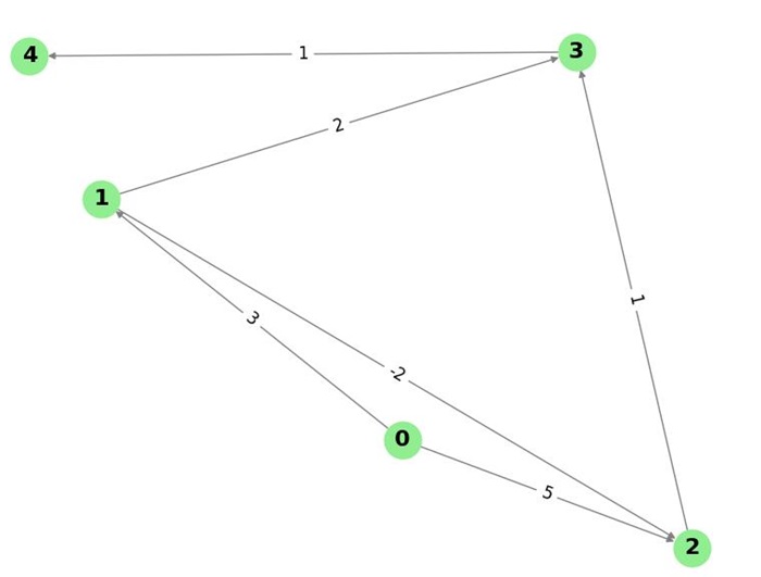
The adjacency list representation of the graph is as follows −
graph = {
   0: [(1, 3), (2, 5)],
   1: [(2, -2), (3, 2)],
   2: [(3, 1)],
   3: [(4, 1)],
   4: []
}
Let us apply Johnson's algorithm to find the shortest paths between all pairs of vertices in this graph. Here, we will follow each step of the process, from adding a new vertex to the reweighting, executing Dijkstra's algorithm, and recovering the original weights.
Step 1: Add a New Vertex
We add a new vertex q to the graph and connect it to all other vertices with edges of weight 0. The updated graph will look as follows −
graph_with_q = {
   'q': [(0, 0), (1, 0), (2, 0), (3, 0), (4, 0)],
   0: [(1, 3), (2, 5)],
   1: [(2, -2), (3, 2)],
   2: [(3, 1)],
   3: [(4, 1)],
   4: []
}
Step 2: Apply Bellman-Ford Algorithm
Next, we run the Bellman-Ford algorithm from the newly added vertex q to calculate the shortest distances from q to every other vertex.
The Bellman-Ford algorithm helps detect negative weight cycles and computes the shortest paths to each vertex. After running Bellman-Ford, we get the shortest path distances from q to all other vertices:
h = {
   'q': 0,
   0: 0,
   1: 3,
   2: 5,
   3: 6,
   4: 7
}
Step 3: Reweight the Edges
We then reweight the edges using the formula −
new_weight(u, v) = original_weight(u, v) + h(u) - h(v)
This ensures that all edge weights are non-negative. The reweighted graph looks like this:
reweighted_graph = {
   0: [(1, 0), (2, 3)],
   1: [(2, -5), (3, 1)],
   2: [(3, -5)],
   3: [(4, -6)],
   4: []
}
Step 4: Run Dijkstra's Algorithm
Now that all edge weights are non-negative, we can use Dijkstra's algorithm to find the shortest paths from each vertex to all other vertices. We will run Dijkstra's algorithm for each vertex in the graph:
import heapq

def dijkstra(graph, start):
   dist = {vertex: float('inf') for vertex in graph}
   dist[start] = 0
   priority_queue = [(0, start)]

   while priority_queue:
      current_distance, current_vertex = heapq.heappop(priority_queue)

      if current_distance > dist[current_vertex]:
         continue

      for neighbor, weight in graph[current_vertex]:
         distance = current_distance + weight
         if distance < dist[neighbor]:
            dist[neighbor] = distance
            heapq.heappush(priority_queue, (distance, neighbor))

   return dist

# Running Dijkstra for all vertices
all_pairs_shortest_paths = {}
for vertex in graph_with_q:
   all_pairs_shortest_paths[vertex] = dijkstra(reweighted_graph, vertex)

print(all_pairs_shortest_paths)
Step 5: Recover the Original Weights
After running Dijkstra's algorithm, we adjust the results back to the original edge weights by subtracting the reweighting factors:
adjusted_paths = {}
for start in all_pairs_shortest_paths:
   adjusted_paths[start] = {}
   for end in all_pairs_shortest_paths[start]:
      adjusted_paths[start][end] = all_pairs_shortest_paths[start][end] + h[end] - h[start]

print(adjusted_paths)
Complete Implementation
Following is a Python complete implementation of Johnson's algorithm −
graph = {
   0: [(1, 3), (2, 5)],
   1: [(2, -2), (3, 2)],
   2: [(3, 1)],
   3: [(4, 1)],
   4: []
}
graph_with_q = {
   'q': [(0, 0), (1, 0), (2, 0), (3, 0), (4, 0)],
   0: [(1, 3), (2, 5)],
   1: [(2, -2), (3, 2)],
   2: [(3, 1)],
   3: [(4, 1)],
   4: []
}
h = {
   'q': 0,
   0: 0,
   1: 3,
   2: 5,
   3: 6,
   4: 7
}
reweighted_graph = {
   'q': [(0, 0), (1, 0), (2, 0), (3, 0), (4, 0)],
   0: [(1, 0), (2, 3)],
   1: [(2, -5), (3, 1)],
   2: [(3, -5)],
   3: [(4, -6)],
   4: []
}

import heapq

def dijkstra(graph, start):
   dist = {vertex: float('inf') for vertex in graph}
   dist[start] = 0
   priority_queue = [(0, start)]

   while priority_queue:
      current_distance, current_vertex = heapq.heappop(priority_queue)

      if current_distance > dist[current_vertex]:
         continue

      for neighbor, weight in graph[current_vertex]:
         distance = current_distance + weight
         if distance < dist[neighbor]:
            dist[neighbor] = distance
            heapq.heappush(priority_queue, (distance, neighbor))

   return dist

# Printing the Original Graph
print("Original Graph::")
print(graph)

# Printing the Reweighted Graph
print("\nReweighted Graph::")
print(reweighted_graph)

# Running Dijkstra for all vertices
all_pairs_shortest_paths = {}
for vertex in graph_with_q:
   all_pairs_shortest_paths[vertex] = dijkstra(reweighted_graph, vertex)

# Printing All Pairs Shortest Paths
print("\nAll Pairs Shortest Paths:")
print(all_pairs_shortest_paths)

# Adjusting the shortest paths using the potential function h
adjusted_paths = {}
for start in all_pairs_shortest_paths:
   adjusted_paths[start] = {}
   for end in all_pairs_shortest_paths[start]:
      adjusted_paths[start][end] = all_pairs_shortest_paths[start][end] + h[end] - h[start]

# Printing Adjusted Shortest Paths
print("\nAdjusted Shortest Paths:")
print(adjusted_paths)
This produces the following output −
Original Graph::
{0: [(1, 3), (2, 5)], 1: [(2, -2), (3, 2)], 2: [(3, 1)], 3: [(4, 1)], 4: []}

Reweighted Graph::
{'q': [(0, 0), (1, 0), (2, 0), (3, 0), (4, 0)], 0: [(1, 0), (2, 3)], 1: [(2, -5), (3, 1)], 2: [(3, -5)], 3: [(4, -6)], 4: []}
All Pairs Shortest Paths:
{'q': {'q': 0, 0: 0, 1: 0, 2: -5, 3: -10, 4: -16}, 0: {'q': inf, 0: 0, 1: 0, 2: -5, 3: -10, 4: -16}, 1: {'q': inf, 0: inf, 1: 0, 2: -5, 3: -10, 4: -16}, 2: {'q': inf, 0: inf, 1: inf, 2: 0, 3: -5, 4: -11}, 3: {'q': inf, 0: inf, 1: inf, 2: inf, 3: 0, 4: -6}, 4: {'q': inf, 0: inf, 1: inf, 2: inf, 3: inf, 4: 0}}

Adjusted Shortest Paths:
{'q': {'q': 0, 0: 0, 1: 3, 2: 0, 3: -4, 4: -9}, 0: {'q': inf, 0: 0, 1: 3, 2: 0, 3: -4, 4: -9}, 1: {'q': inf, 0: inf, 1: 0, 2: -3, 3: -7, 4: -12}, 2: {'q': inf, 0: inf, 1: inf, 2: 0, 3: -4, 4: -9}, 3: {'q': inf, 0: inf, 1: inf, 2: inf, 3: 0, 4: -5}, 4: {'q': inf, 0: inf, 1: inf, 2: inf, 3: inf, 4: 0}}

Complexity of Johnson's Algorithm
The time complexity of Johnson's algorithm is O(V2 log V + VE), where V is the number of vertices and E is the number of edges in the graph. The most time-consuming part is running Dijkstra's algorithm for each vertex, which has a time complexity of O(E log V) for each run.
The space complexity of Johnson's algorithm is O(V2 + E) because it requires storing the adjacency list representation of the graph, the reweighted graph, and the distances computed by Dijkstra's algorithm.
Applications of Johnson's Algorithm
Johnson's algorithm has various applications, including:
- All-Pairs Shortest Path: Johnson's algorithm is used to find the shortest paths between all pairs of vertices, especially in sparse graphs.
- Network Analysis: It is useful in network routing problems where we need to compute the shortest paths between multiple nodes in a network.
- Optimal Pathfinding: It is used in situations where finding the optimal path from multiple sources to multiple destinations is required, such as in transportation or logistics problems.
- Pathfinding in Large Graphs: Johnson's algorithm is useful in handling large graphs where the number of edges is much smaller than the square of the number of vertices.
