Graph Theory - Graph Algorithms

---

---

Graph Algorithms

Graph algorithms are a set of algorithms used to solve problems that involve graph structures. A graph consists of vertices (or nodes) and edges (or arcs) that connect pairs of vertices. A graph can be represented in various forms, such as an adjacency matrix, adjacency list, or edge list.

Graph algorithms help solve problems related to graph traversal, searching, or finding specific characteristics or properties within the graph.

They are widely used in various fields, such as computer science, mathematics, network analysis, and artificial intelligence.

Some of the common tasks that graph algorithms can perform are as follows −

• Finding the shortest path between two vertices
• Finding the minimum spanning tree
• Detecting cycles in a graph
• Determining connectivity between nodes
• Graph coloring and bipartiteness checking

Types of Graphs in Graph Algorithms

Before learning about specific algorithms, it is important to understand the different types of graphs that are present in graph theory. These include −

• Directed Graphs (Digraphs): In these graphs, edges have a direction, meaning each edge has a starting and ending vertex.
• Undirected Graphs: In these graphs, edges have no direction, meaning the edge can be traversed in either direction.
• Weighted Graphs: In these graphs, edges have weights (or costs) associated with them, often used in algorithms like Dijkstra's and Prim's.
• Unweighted Graphs: In these graphs, edges do not have weights and are typically used in basic traversal algorithms.
• Cyclic Graphs: Graphs that contain at least one cycle (a path from a vertex back to itself).
• Acyclic Graphs: Graphs that do not contain cycles. Directed Acyclic Graphs (DAGs) are commonly used in dependency resolution and scheduling problems.

Graph Traversal Algorithms

Graph traversal is the process of visiting all the vertices or edges in a graph. There are two primary methods for graph traversal −

• Depth-First Search (DFS): This algorithm starts at a source vertex and explores as far as possible along each branch before backtracking. DFS is useful for tasks like cycle detection and topological sorting.
• Breadth-First Search (BFS): This algorithm starts at a source vertex and explores all neighboring vertices at the present depth level before moving on to the next level. BFS is commonly used for finding the shortest path in unweighted graphs.

Depth-First Search

DFS is a graph traversal algorithm that explores as far as possible along each branch before backtracking. It uses a stack (or recursion) to keep track of vertices to be explored. DFS can be used to −

• Traverse all vertices in a connected graph
• Detect cycles in a graph
• Find a path between two vertices
• Perform topological sorting in directed acyclic graphs (DAGs)

The above image displays all vertices reachable from the starting vertex −

Visiting vertex 0
Going deeper to vertex 1
Visiting vertex 1
Going deeper to vertex 3
Visiting vertex 3
Going deeper to vertex 4
Visiting vertex 4
Going deeper to vertex 2
Visiting vertex 2
All visited vertices: {0, 1, 2, 3, 4}

Breadth-First Search

BFS is another graph traversal algorithm that explores the graph level by level, starting from the source vertex. It is implemented using a queue to manage the frontier of vertices to explore. BFS is commonly used in −

• Finding the shortest path in unweighted graphs
• Checking graph bipartiteness
• Searching for the connected components of a graph

In the above given graph, following is the BFS traversal −

Starting BFS from vertex 0
Visiting vertex 0
Adding vertex 1 to the queue
Adding vertex 2 to the queue
Visiting vertex 1
Adding vertex 3 to the queue
Adding vertex 4 to the queue
Visiting vertex 2
Visiting vertex 3
Visiting vertex 4
All visited vertices: {0, 1, 2, 3, 4}

Shortest Path Algorithms

Finding the shortest path between two vertices in a graph is a fundamental problem in graph theory. We can use different algorithms depending on whether the graph is weighted or unweighted. The two main algorithms for finding the shortest path are −

• Dijkstra's Algorithm: This algorithm finds the shortest path from a source vertex to all other vertices in a weighted graph. It is used when all edge weights are non-negative.
• Bellman-Ford Algorithm: This algorithm also finds the shortest path from a source vertex to all other vertices but works with graphs that may have negative edge weights.

Dijkstra's Algorithm

Dijkstra's algorithm is a greedy algorithm that calculates the shortest path from a source vertex to all other vertices in a weighted graph with non-negative edge weights. It maintains a priority queue (min-heap) to select the vertex with the minimum distance at each step.

In the following image, we use Dijkstra's algorithm to find the shortest path from vertex A to vertex F in a weighted graph −

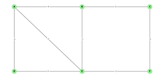
The shortest path from A to F using Dijkstra's algorithm is A - E - F with a total weight of 2.

Bellman-Ford Algorithm

The Bellman-Ford algorithm is used to find the shortest path in a graph that may contain negative weights. Unlike Dijkstra's algorithm, Bellman-Ford can handle negative edges and also detects negative-weight cycles in the graph.

The following image displays the shortest distances from vertex 0 to all other vertices in the graph, while also checking for negative-weight cycles −

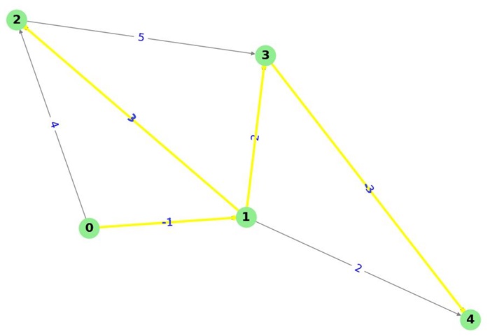
Here, we find the shortest distances from the source vertex 0 to all other vertices. The resulting shortest distances are as follows −

• Vertex 0: The distance to itself is 0, as no travel is needed.
• Vertex 1: The shortest distance is -1, achieved via the edge from vertex 0 to vertex 1 with a weight of -1.
• Vertex 2: The shortest distance is 2, found by traveling from vertex 0 to vertex 1 (distance -1), and then from vertex 1 to vertex 2 (distance 3), resulting in a total distance of -1 + 3 = 2.
• Vertex 3: The shortest distance is 1, obtained by traveling from vertex 0 to vertex 1 (distance -1), and then from vertex 1 to vertex 3 (distance 2), resulting in a total distance of -1 + 2 = 1.
• Vertex 4: The shortest distance is -2, found by traveling from vertex 0 to vertex 1 (distance -1), from vertex 1 to vertex 4 (distance 2), and then from vertex 3 to vertex 4 (distance -3), resulting in a total distance of -1 + 2 - 3 = -2.

Hence, shortest distances from vertex 0: {0: 0, 1: -1, 2: 2, 3: 1, 4: -2}

Minimum Spanning Tree Algorithms

A Minimum Spanning Tree (MST) is a subgraph of an undirected, weighted graph that connects all the vertices together with the minimum total edge weight, without any cycles. There are two commonly used algorithms to find an MST −

• Kruskal's Algorithm: This algorithm sorts the edges by weight and adds them one by one to the MST, ensuring that no cycles are formed.
• Prim's Algorithm: This algorithm grows the MST by adding the minimum weight edge from the tree to a vertex not yet in the tree, repeating until all vertices are connected.

In the above image −

MST Edges: [('A', 'D', {'weight': 2}), ('A', 'B', {'weight': 3}), ('B', 'C', {'weight': 1})]

Kruskal's Algorithm

Kruskal's algorithm is a greedy algorithm used to find the MST of a graph. It works by sorting the edges by weight and adding edges to the MST in increasing order of weight, ensuring no cycles are formed.

Prim's Algorithm

Prim's algorithm starts with any vertex and grows the minimum spanning tree (MST) by adding one vertex at a time. It always adds the smallest edge that connects a vertex already in the tree to a vertex not yet in the tree. A priority queue is used to select the smallest edge at each step.

Cycle Detection Algorithms

Cycle detection is the process of finding cycles (if any) in a graph. It is important in tasks such as checking dependencies in directed graphs and detecting infinite loops. The two major methods for cycle detection are −

• DFS-Based Cycle Detection: This method uses DFS to explore the graph and keep track of the visited vertices. If a vertex is encountered that is already in the recursion stack, a cycle is detected.
• Union-Find Cycle Detection: This method uses a union-find data structure to keep track of connected components and detect cycles in an undirected graph.

DFS-Based Cycle Detection

DFS-based cycle detection uses a depth-first search to explore the graph and keep track of the vertices in the recursion stack. If a vertex is encountered that is already in the recursion stack, a cycle is detected.

The following image shows an example of DFS-based cycle detection −

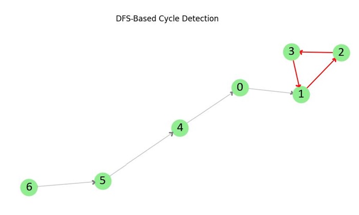
In this graph, a cycle is detected involving vertices 1, 2, and 3.

Union-Find Cycle Detection

Union-find cycle detection uses a union-find data structure to keep track of connected components in an undirected graph. If adding an edge connects two vertices that are already in the same component, a cycle is detected.

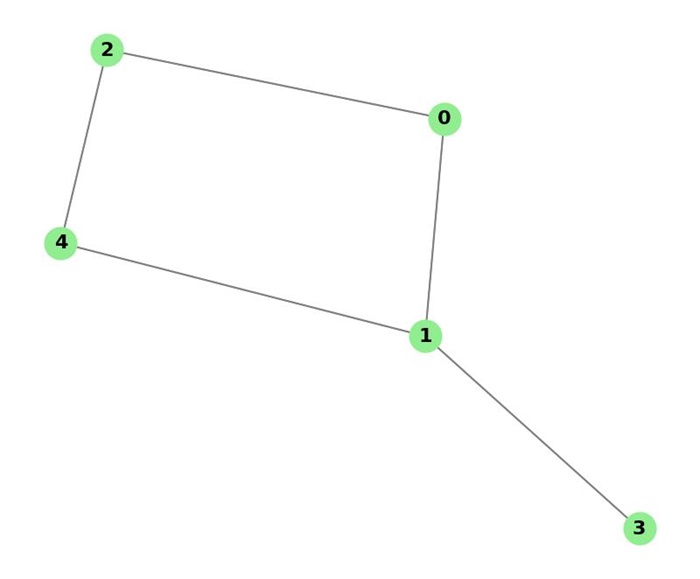
The following image shows an example of union-find cycle detection −

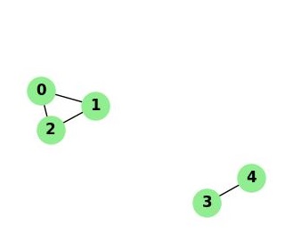
In this graph, a cycle is detected with vertices 0, 1, and 2.

Graph Coloring Algorithms

Graph coloring is the task of assigning colors to the vertices of a graph so that no two adjacent vertices have the same color. It is used in various applications, such as scheduling and register allocation in compilers. The two main graph coloring algorithms are −

• Greedy Coloring Algorithm: A simple algorithm that assigns the smallest possible color to each vertex in a greedy manner.
• Backtracking Algorithm: A more sophisticated algorithm that uses backtracking to find an optimal coloring.

Greedy Coloring Algorithm

The Greedy Coloring Algorithm assign a color to each vertex of a graph such that no two adjacent vertices have the same color. The algorithm works by choosing the first available color for each vertex, starting from one vertex and moving on to the next.

It is called "greedy" because it makes the locally optimal choice (assigning a color that hasn't been used by its neighbors) at each step, without considering the bigger picture or future moves.

The following image shows an example of greedy coloring −

In this graph, the greedy algorithm assigns colors such that no two adjacent vertices have the same color.

Backtracking Coloring Algorithm

The Backtracking Coloring Algorithm is a more advanced method for coloring the vertices of a graph. It is used to assign colors to the vertices such that no two adjacent vertices have the same color.

It works by trying to color a vertex with a color and then moving on to the next vertex. If it finds a conflict (two adjacent vertices having the same color), it "backtracks" to the previous vertex and tries a different color. This process continues until all vertices are colored correctly or until it determines that no solution is possible.

Connected Components Algorithms

Finding the connected components of a graph means identifying all the subgraphs in which any two vertices are connected to each other by paths, and which are not connected to other vertices. The two main algorithms for finding connected components are −

• DFS-Based Connected Components: This method uses DFS to explore the graph and identify connected components.
• BFS-Based Connected Components: This method uses BFS to explore the graph and identify connected components.

DFS-Based Connected Components

DFS-based connected components use depth-first search to explore the graph and identify all the connected components. It starts from each unvisited vertex and performs a DFS to mark all reachable vertices as part of the same component.

The following image shows an example of DFS-based connected components −

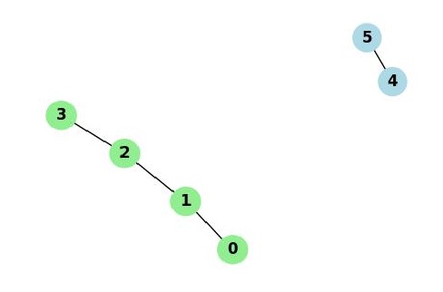
In this graph, DFS identifies two connected components: {0, 1, 2, 3} and {4, 5}.

BFS-Based Connected Components

BFS-based connected components use breadth-first search to explore the graph and identify all the connected components. It starts from each unvisited vertex and performs a BFS to mark all reachable vertices as part of the same component.