Graph Theory - Branchwidth

---

---

Branchwidth

Branchwidth is a graph parameter that measures how close a graph is to being a tree in terms of its edge connectivity. It is closely related to the concept of treewidth but focuses on the structure of the graph's edges rather than its vertices.

• A tree has a branchwidth of 1 because there is only one way to connect its nodes with edges.
• Graphs with many edges or high connectivity have a higher branchwidth.

The branchwidth of a graph G is defined as the minimum branchwidth among all branch decompositions of G. A branch decomposition is a way of representing a graph as a tree, where the nodes correspond to edges of the graph, and the edges of the tree represent relationships between these edges.

Branchwidth is similar to treewidth but with a different perspective ‐ it is focused on how edges are grouped in a tree-like structure rather than the vertices.

Importance of Branchwidth

Branchwidth plays an important role in various graph-related problems. It helps in designing algorithms for problems related to connectivity and edge partitioning −

• Better Algorithms: Many edge-based problems become easier to solve on graphs with small branchwidth.
• Graph Decomposition: Branchwidth helps in decomposing graphs into simpler components for more quick analysis.
• Connectivity Analysis: It helps in understanding the connectivity structure of graphs, which is important in network design.
• Applications in Network Theory: Branchwidth is used to analyze and optimize network structures and routing algorithms.

Branch Decompositions and Branchwidth

A branch decomposition represents a graph in a tree-like structure, where −

• Each node of the tree corresponds to an edge of the graph.
• For each pair of adjacent edges in the graph, there must be at least one tree node connecting them.
• Each node's "bag" consists of a set of edges that form a connected subset of the graph.

The branchwidth of the graph is determined by finding the minimum size of the largest bag minus one over all possible branch decompositions −

Branchwidth = min(|Bag|) - 1

Example of Branchwidth Calculation

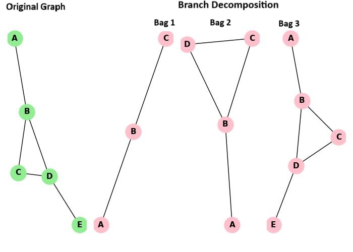
Consider the following graph −

Graph:
Edges = [(A, B), (B, C), (C, D), (B, D), (D, E)]

A branch decomposition of this graph might look like this −

Branch Decomposition:
Bag 1: [(A, B), (B, C)]
Bag 2: [(B, D), (C, D)]
Bag 3: [(D, E)]

The size of the largest bag is 2, so the branchwidth is −

Branchwidth = 2 - 1 = 1

Properties of Branchwidth

Graphs with small branchwidth have the following properties −

• Edge Partitioning: A graph with low branchwidth allows for effective partitioning of edges into manageable subsets.
• Efficient Algorithms: Many edge-based algorithms perform better on graphs with low branchwidth.
• Tree-like Edge Structure: Graphs with small branchwidth have a structure that is similar to tree connectivity.
• Multiple Decompositions: A graph may have many different branch decompositions, each with a different branchwidth.

Graphs with Bounded Branchwidth

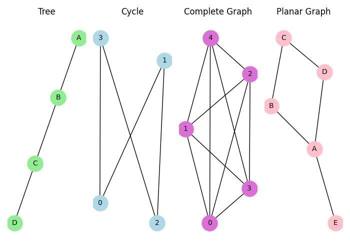
Some classes of graphs have bounded branchwidth. These include −

• Trees: A tree has a branchwidth of 1 because it only has one connection between any two nodes.
• Cycles: A cycle graph has a branchwidth of 2, as every edge in the cycle is part of a bag of size 2.
• Complete Graphs: A complete graph with n vertices has a branchwidth that grows as the number of vertices increases.
• Planar Graphs: Planar graphs, which can be drawn on a plane without edges crossing, have various branchwidths depending on the specific graph structure.

Branchwidth and Computational Problems

The following problems can benefit from graphs with low branchwidth −

• Graph Cut Problems: Solving graph partitioning and cut problems is more efficient on graphs with low branchwidth.
• Network Reliability: The connectivity of networks are easier to analyze when the branchwidth is small.
• Graph Coloring: Finding optimal colorings of a graph becomes easier when the branchwidth is minimized.
• Pathfinding Problems: Algorithms for finding paths, such as the shortest path problem, work faster on graphs with small branchwidth.

Example: Algorithm Using Branchwidth

Let us implement an algorithm to find the optimal edge partitioning on a graph using its branchwidth. We will use dynamic programming to break down the problem into manageable subproblems, based on the branch decomposition.

# Graph Definition
Edges = [("A", "B"), ("B", "C"), ("C", "D"), ("D", "E")]

# Branch Decomposition
Branch_Decomposition = {
    1: [("A", "B"), ("B", "C")],
    2: [("B", "D"), ("C", "D")],
    3: [("D", "E")]
}

# Initialize a dictionary to store the optimal edge partitions
Edge_Partition = {}

# Iterate through each bag in the branch decomposition
for bag in Branch_Decomposition.values():
   # For each edge in the current bag, compute the optimal partition
   for edge in bag:
      # Update the edge partitioning for the edge
      Edge_Partition[edge] = "Optimal Partition"
        
# Output the optimal edge partitions for each edge
print(Edge_Partition)

We get the output as shown below −

{('A', 'B'): 'Optimal Partition', ('B', 'C'): 'Optimal Partition', ('B', 'D'): 'Optimal Partition', ('C', 'D'): 'Optimal Partition', ('D', 'E'): 'Optimal Partition'}