- Graph Theory - Home
- Graph Theory - Introduction
- Graph Theory - History
- Graph Theory - Fundamentals
- Graph Theory - Applications
- Types of Graphs
- Graph Theory - Types of Graphs
- Graph Theory - Simple Graphs
- Graph Theory - Multi-graphs
- Graph Theory - Directed Graphs
- Graph Theory - Weighted Graphs
- Graph Theory - Bipartite Graphs
- Graph Theory - Complete Graphs
- Graph Theory - Subgraphs
- Graph Theory - Trees
- Graph Theory - Forests
- Graph Theory - Planar Graphs
- Graph Theory - Hypergraphs
- Graph Theory - Infinite Graphs
- Graph Theory - Random Graphs
- Graph Representation
- Graph Theory - Graph Representation
- Graph Theory - Adjacency Matrix
- Graph Theory - Adjacency List
- Graph Theory - Incidence Matrix
- Graph Theory - Edge List
- Graph Theory - Compact Representation
- Graph Theory - Incidence Structure
- Graph Theory - Matrix-Tree Theorem
- Graph Properties
- Graph Theory - Basic Properties
- Graph Theory - Coverings
- Graph Theory - Matchings
- Graph Theory - Independent Sets
- Graph Theory - Traversability
- Graph Theory Connectivity
- Graph Theory - Connectivity
- Graph Theory - Vertex Connectivity
- Graph Theory - Edge Connectivity
- Graph Theory - k-Connected Graphs
- Graph Theory - 2-Vertex-Connected Graphs
- Graph Theory - 2-Edge-Connected Graphs
- Graph Theory - Strongly Connected Graphs
- Graph Theory - Weakly Connected Graphs
- Graph Theory - Connectivity in Planar Graphs
- Graph Theory - Connectivity in Dynamic Graphs
- Special Graphs
- Graph Theory - Regular Graphs
- Graph Theory - Complete Bipartite Graphs
- Graph Theory - Chordal Graphs
- Graph Theory - Line Graphs
- Graph Theory - Complement Graphs
- Graph Theory - Graph Products
- Graph Theory - Petersen Graph
- Graph Theory - Cayley Graphs
- Graph Theory - De Bruijn Graphs
- Graph Algorithms
- Graph Theory - Graph Algorithms
- Graph Theory - Breadth-First Search
- Graph Theory - Depth-First Search (DFS)
- Graph Theory - Dijkstra's Algorithm
- Graph Theory - Bellman-Ford Algorithm
- Graph Theory - Floyd-Warshall Algorithm
- Graph Theory - Johnson's Algorithm
- Graph Theory - A* Search Algorithm
- Graph Theory - Kruskal's Algorithm
- Graph Theory - Prim's Algorithm
- Graph Theory - Borůvka's Algorithm
- Graph Theory - Ford-Fulkerson Algorithm
- Graph Theory - Edmonds-Karp Algorithm
- Graph Theory - Push-Relabel Algorithm
- Graph Theory - Dinic's Algorithm
- Graph Theory - Hopcroft-Karp Algorithm
- Graph Theory - Tarjan's Algorithm
- Graph Theory - Kosaraju's Algorithm
- Graph Theory - Karger's Algorithm
- Graph Coloring
- Graph Theory - Coloring
- Graph Theory - Edge Coloring
- Graph Theory - Total Coloring
- Graph Theory - Greedy Coloring
- Graph Theory - Four Color Theorem
- Graph Theory - Coloring Bipartite Graphs
- Graph Theory - List Coloring
- Advanced Topics of Graph Theory
- Graph Theory - Chromatic Number
- Graph Theory - Chromatic Polynomial
- Graph Theory - Graph Labeling
- Graph Theory - Planarity & Kuratowski's Theorem
- Graph Theory - Planarity Testing Algorithms
- Graph Theory - Graph Embedding
- Graph Theory - Graph Minors
- Graph Theory - Isomorphism
- Spectral Graph Theory
- Graph Theory - Graph Laplacians
- Graph Theory - Cheeger's Inequality
- Graph Theory - Graph Clustering
- Graph Theory - Graph Partitioning
- Graph Theory - Tree Decomposition
- Graph Theory - Treewidth
- Graph Theory - Branchwidth
- Graph Theory - Graph Drawings
- Graph Theory - Force-Directed Methods
- Graph Theory - Layered Graph Drawing
- Graph Theory - Orthogonal Graph Drawing
- Graph Theory - Examples
- Computational Complexity of Graph
- Graph Theory - Time Complexity
- Graph Theory - Space Complexity
- Graph Theory - NP-Complete Problems
- Graph Theory - Approximation Algorithms
- Graph Theory - Parallel & Distributed Algorithms
- Graph Theory - Algorithm Optimization
- Graphs in Computer Science
- Graph Theory - Data Structures for Graphs
- Graph Theory - Graph Implementations
- Graph Theory - Graph Databases
- Graph Theory - Query Languages
- Graph Algorithms in Machine Learning
- Graph Neural Networks
- Graph Theory - Link Prediction
- Graph-Based Clustering
- Graph Theory - PageRank Algorithm
- Graph Theory - HITS Algorithm
- Graph Theory - Social Network Analysis
- Graph Theory - Centrality Measures
- Graph Theory - Community Detection
- Graph Theory - Influence Maximization
- Graph Theory - Graph Compression
- Graph Theory Real-World Applications
- Graph Theory - Network Routing
- Graph Theory - Traffic Flow
- Graph Theory - Web Crawling Data Structures
- Graph Theory - Computer Vision
- Graph Theory - Recommendation Systems
- Graph Theory - Biological Networks
- Graph Theory - Social Networks
- Graph Theory - Smart Grids
- Graph Theory - Telecommunications
- Graph Theory - Knowledge Graphs
- Graph Theory - Game Theory
- Graph Theory - Urban Planning
- Graph Theory Useful Resources
- Graph Theory - Quick Guide
- Graph Theory - Useful Resources
- Graph Theory - Discussion
Graph Theory - Edmonds-Karp Algorithm
Edmonds-Karp Algorithm
The Edmonds-Karp algorithm is an implementation of the Ford-Fulkerson method for computing the maximum flow in a flow network. It uses breadth-first search (BFS) to find augmenting paths in the residual graph, ensuring that the shortest augmenting path is found in each iteration.
An augmenting path is a path from the source to the sink where every edge in the path has a positive residual capacity (i.e., the flow can still be increased along the edge).
This improves the performance of the basic Ford-Fulkerson algorithm by providing a more structured method for searching augmenting paths. The algorithm guarantees finding the maximum flow in polynomial time, specifically in O(VE2), where V is the number of vertices and E is the number of edges in the graph.
The key difference between Edmonds-Karp and the Ford-Fulkerson algorithm is that Edmonds-Karp always chooses the shortest augmenting path (in terms of the number of edges) by using BFS.
Overview of Edmonds-Karp Algorithm
The Edmonds-Karp algorithm works by finding augmenting paths in the residual graph using breadth-first search (BFS). The main steps of the algorithm are as follows −
- Initialization: Start with a flow of 0 on all edges and construct the residual graph.
- Find Augmenting Path: Use BFS to find the shortest augmenting path in the residual graph.
- Augment Flow: Increase the flow along the found augmenting path by the minimum residual capacity of the edges in the path.
- Update Residual Graph: Update the residual capacities of the edges in the augmenting path.
- Repeat: Repeat the process of finding augmenting paths and updating the flow until no augmenting path exists in the residual graph.
Properties of Edmonds-Karp Algorithm
Edmonds-Karp has several important properties and characteristics that differentiate it from other flow algorithms −
- Polynomial Time: Unlike the basic Ford-Fulkerson algorithm, which can take exponential time in the worst case, the Edmonds-Karp algorithm runs in polynomial time (O(VE2)), where V is the number of vertices and E is the number of edges in the graph.
- Shortest Path Search: The algorithm always finds the shortest augmenting path using breadth-first search (BFS), ensuring efficient flow updates.
- Optimal Flow: The algorithm guarantees the maximum flow solution, just like the Ford-Fulkerson algorithm, by iterating through augmenting paths until no more augmenting paths can be found.
- Capacity Constraints: The algorithm respects the capacity constraints by updating the residual graph after each flow augmentation.
Steps of Edmonds-Karp Algorithm
The steps of the Edmonds-Karp algorithm are as follows −
- Step 1: Initialize Flow: Start with an initial flow of 0 for all edges. The initial flow configuration is often represented as a flow matrix or an adjacency list of flow values.
- Step 2: Construct Residual Graph: Create a residual graph representing the remaining capacity of each edge in the original graph. Initially, the residual capacity of each edge is equal to its capacity in the original graph.
- Step 3: Find Augmenting Path: Use breadth-first search (BFS) to find an augmenting path in the residual graph. This is the shortest path from the source to the sink that still has positive residual capacity along every edge.
- Step 4: Augment Flow: Increase the flow along the found augmenting path. The flow increase is limited by the smallest residual capacity along the path, called the bottleneck capacity.
- Step 5: Update Residual Graph: After augmenting the flow, update the residual graph. The capacity of the forward edges along the path is decreased by the flow amount, and the reverse edges are updated to allow for potential flow reversal.
- Step 6: Repeat: Repeat the process of finding augmenting paths and augmenting the flow until no more augmenting paths exist. When no more augmenting paths are found, the algorithm terminates, and the flow is the maximum flow in the network.
Example of Edmonds-Karp Algorithm
Consider the following graph −
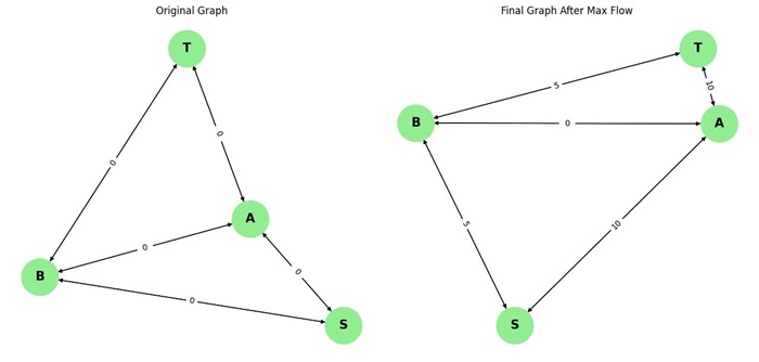
We want to find the maximum flow from the source (S) to the sink (T) using the Edmonds-Karp algorithm.
Step 1: Initialize Flow
Start with an initial flow of 0 on all edges:
flow = {(S, A): 0, (S, B): 0, (A, T): 0, (B, T): 0, (A, B): 0}
Step 2: Find Augmenting Path
In the first iteration, we perform a BFS and find the augmenting path: S A T. The minimum residual capacity along this path is 3 (the capacity of the edge S A).
Step 3: Augment Flow
We augment the flow along this path by 3. After augmenting, the flow becomes:
flow = {(S, A): 3, (S, B): 0, (A, T): 3, (B, T): 0, (A, B): 0}
Step 4: Update Residual Graph
Update the residual capacities:
- Residual Capacity of (S, A): 5 - 3 = 2
- Residual Capacity of (A, T): 3 - 3 = 0
Step 5: Find Augmenting Path Again
In the next iteration, we perform a BFS and find a new augmenting path: S B T. The minimum residual capacity along this path is 2 (the capacity of the edge S B).
Step 6: Augment Flow
We augment the flow by 2 along the path S B T:
flow = {(S, A): 3, (S, B): 2, (A, T): 3, (B, T): 2, (A, B): 0}
Step 7: Update Residual Graph
Update the residual capacities:
- Residual Capacity of (S, B): 4 - 2 = 2
- Residual Capacity of (B, T): 2 - 2 = 0
Step 8: Termination
At this point, no more augmenting paths exist, and the algorithm terminates. The maximum flow in the network is the total flow that has been augmented from the source to the sink. In this case, the maximum flow is 5 (3 + 2).
Complete Python Implementation
Following is the complete Python implementation of the Edmonds-Karp algorithm −
from collections import deque

class Graph:
   def __init__(self, vertices):
      self.V = vertices
      self.graph = {}

   def add_edge(self, u, v, w):
      if u not in self.graph:
         self.graph[u] = {}
      if v not in self.graph:
         self.graph[v] = {}
      self.graph[u][v] = self.graph[u].get(v, 0) + w
	  # Initialize the reverse edge with 0 capacity
      self.graph[v][u] = self.graph[v].get(u, 0)

   def bfs(self, source, sink, parent):
      visited = {key: False for key in self.graph}
      queue = deque([source])
      visited[source] = True

      while queue:
         u = queue.popleft()

         for v in self.graph[u]:
            if not visited[v] and self.graph[u][v] > 0:
               if v == sink:
                  parent[v] = u
                  return True
               queue.append(v)
               parent[v] = u
               visited[v] = True
      return False

   def edmonds_karp(self, source, sink):
      parent = {}
      max_flow = 0

      while self.bfs(source, sink, parent):
         path_flow = float("Inf")
         s = sink
         while s != source:
            path_flow = min(path_flow, self.graph[parent[s]][s])
            s = parent[s]

         max_flow += path_flow
         v = sink
         while v != source:
            u = parent[v]
            self.graph[u][v] -= path_flow
     		# Update the reverse edge capacity
            self.graph[v][u] = self.graph[v].get(u, 0) + path_flow
            v = parent[v]

      return max_flow

# Create a graph and add edges
g = Graph(6)
g.add_edge('S', 'A', 10)
g.add_edge('S', 'B', 5)
g.add_edge('A', 'T', 10)
g.add_edge('B', 'T', 5)
g.add_edge('A', 'B', 15)

# Find the maximum flow
max_flow = g.edmonds_karp('S', 'T')
print("The maximum possible flow is", max_flow)
Following is the output obtained −
The maximum possible flow is 15
Complexity Analysis
The time complexity of the Edmonds-Karp algorithm is O(VE2), where V is the number of vertices and E is the number of edges in the graph. This is because the algorithm performs a breadth-first search (BFS) to find augmenting paths, and each augmenting path requires at most O(E) time.
The algorithm performs at most O(VE) augmentations, leading to the overall time complexity.
The space complexity is O(V + E) due to the storage of the graph and the parent array used for BFS.
