Graph Theory - Graph Clustering

---

---

Graph Clustering

Graph Clustering is a process of dividing the nodes of a graph into groups or clusters such that nodes within the same group are highly connected, while nodes in different groups have fewer connections.

The goal is to maximize the density of edges within clusters while minimizing the edges between different clusters.

The above graph visualizes graph clustering at three stages −

• Original Graph: The graph with no clustering applied.
• Intermediate Clustering: A state where clustering has partially separated nodes into smaller groups.
• Final Clusters: The final clustered state showing distinct groups.

Properties of Graph Clustering

Following are the properties of graph clustering −

• Intra-Cluster Connectivity: Nodes within the same cluster should have high connectivity or similarity.
• Inter-Cluster Sparsity: Connections between nodes in different clusters should be minimal.
• Balance: The sizes of the clusters should be balanced, avoiding clusters that are too large or too small.

Modularity-Based Clustering

Modularity-Based Clustering is a method used to identify communities or clusters within a graph by maximizing a metric called modularity. Modularity measures the density of edges within clusters compared to edges between clusters.

The modularity value ranges from -1 to 1, where higher modularity values indicate better-defined clusters with more internal connections and fewer external ones.

Example

Consider a graph with the following adjacency matrix −

Adjacency matrix A:
[[0, 1, 1, 0, 0],
 [1, 0, 1, 1, 0],
 [1, 1, 0, 0, 0],
 [0, 1, 0, 0, 1],
 [0, 0, 0, 1, 0]]

Using a modularity-based algorithm, we can divide the graph into two clusters −

• Cluster 1: Nodes {0, 1, 2}
• Cluster 2: Nodes {3, 4}

The modularity score for this clustering is 0.22, indicating a reasonably good partition.

Spectral Clustering

Spectral Clustering is a technique used to group data points into clusters by analyzing the eigenvalues (spectra) of the similarity matrix of a graph. It works by transforming the graph into a matrix, usually the Laplacian matrix, and then computing its eigenvectors.

The eigenvectors are then used to reduce the dimensionality of the data, which is followed by clustering, generally using k-means. Spectral clustering is effective in identifying clusters of arbitrary shapes and works well even when the data is not linearly separable.

Example

For the same graph, spectral clustering involves computing the Laplacian matrix, finding its eigenvalues and eigenvectors, and using the eigenvectors for clustering. The resulting clusters are −

• Cluster 1: Nodes {0, 1, 2}
• Cluster 2: Nodes {3, 4}

Spectral clustering provides a similar result to modularity-based clustering in this case.

The Laplacian matrix is computed using the formula L = D A, where D is the degree matrix and A is the adjacency matrix.

Hierarchical Clustering

Hierarchical clustering builds a hierarchy of clusters by iteratively merging or splitting clusters based on similarity or connectivity. It is divided into two main types −

• Agglomerative: It starts with each node as a separate cluster and merges the closest clusters at each step.
• Divisive: It starts with a single cluster containing all nodes and splits them into smaller clusters iteratively.

The result of hierarchical clustering is usually represented as a dendrogram, a tree-like diagram that shows the merging or splitting process. This method is useful for visualizing the relationships between nodes and determining the number of clusters.

Example

Using an agglomerative approach, we start with each node as a separate cluster and iteratively merge them based on their connectivity. The resulting dendrogram shows the hierarchy of clusters, which can be cut at a specific level to obtain −

• Cluster 1: Nodes {1, 2, 3}
• Cluster 2: Nodes {4, 5}

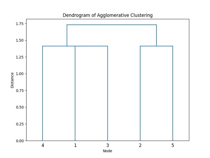
Merging clusters [1] and [3] into [1, 3]
Merging clusters [4] and [1, 3] into [4, 1, 3]
Merging clusters [2] and [5] into [1, 5]
Merging clusters [4, 1, 3] and [2, 5] into [4, 1, 3, 2, 5]

Random Walk Clustering

Random Walk Clustering is technique based on the idea of simulating random walks on a graph. In this approach, data points are represented as nodes in a graph, and edges between nodes represent relationships or similarities between them.

The algorithm assigns clusters by analyzing how random walks transition between nodes. Nodes that are frequently visited together during a random walk are grouped into the same cluster. Random Walk Clustering provides the structure of the graph to discover clusters of data that are closely related.

Applications of Graph Clustering

Graph clustering has several applications across various domains −

• Social Network Analysis: Identifying communities or groups within social networks.
• Biological Networks: Discovering functional modules in protein interaction networks.
• Recommendation Systems: Grouping users with similar preferences for personalized recommendations.
• Web Graphs: Identifying clusters of related web pages for better search engine optimization.