Graph Theory - Graph Diameter

---

---

Graph Diameter

The diameter of a graph is the greatest distance between any pair of vertices, where the distance between two vertices is defined as the length of the shortest path connecting them.

In mathematical terms, the diameter of a graph G is denoted as diam(G). If d(u, v) represents the shortest path distance between vertices u and v, the diameter is given by −

diam(G) = max(d(u, v)) for all u, v in G

This means that the diameter is the maximum value among all the shortest path distances between any two vertices in the graph.

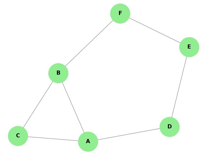
In this graph, the shortest path distances between pairs of vertices are as follows −

• d(A, B) = 1
• d(A, C) = 1
• d(A, D) = 1
• d(A, E) = 2
• d(A, F) = 2
• d(B, C) = 1
• d(B, D) = 2
• d(B, E) = 2
• d(B, F) = 1
• d(C, D) = 2
• d(C, E) = 3
• d(C, F) = 2
• d(D, E) = 1
• d(D, F) = 2
• d(E, F) = 1

The diameter of this graph is 3, which is the longest shortest path between vertices C and E.

Computing the Diameter

We can use various algorithms to compute the diameter of the graph, such as −

• Floyd-Warshall Algorithm
• Breadth-First Search (BFS) Algorithm
• Dijkstra's Algorithm

Floyd-Warshall Algorithm

The Floyd-Warshall algorithm is used to find shortest paths between all pairs of vertices in a graph. It has a time complexity of O(V³), where V is the number of vertices.

In the following graph, we use the Floyd-Warshall algorithm to compute the diameter of a graph −

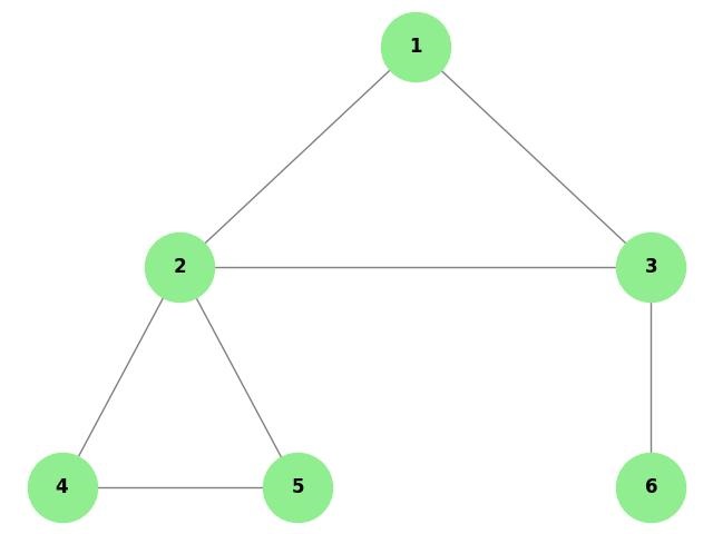
The diameter of the graph is 3 because the longest shortest path between any two vertices in the graph is from node 4 to node 6, passing through nodes 2 and 3. This path has a total length of 3 edges.

Breadth-First Search (BFS)

BFS can be used to find the shortest path between vertices in an unweighted graph. To compute the diameter using BFS, we perform a BFS from each vertex and record the maximum distance found.

In the following example, we use BFS to compute the diameter of an unweighted graph −

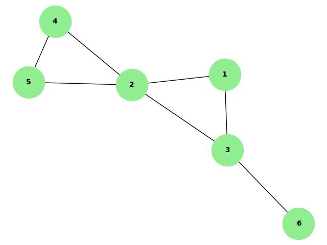
The diameter of the graph is 3. This is because the longest shortest path between any two vertices in the graph is from vertex 1 to vertex 4, passing through vertices 2 and 5.

Graph Diameter: Simple Undirected Graph

The diameter of a simple undirected graph is the longest shortest path between any two nodes in the graph. It measures the maximum distance you need to travel to connect any two nodes.

A simple undirected path is a sequence of distinct nodes in an undirected graph where each node is connected to the next one by an edge, and no node is repeated in the path. In other words, it is a path that doesn't revisit any node, and the edges have no direction, meaning the connection between nodes can be traversed in both directions.

Consider the following simple undirected graph −

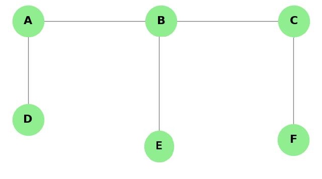
The shortest path distances between pairs of vertices are as follows −

• d(A, B) = 1
• d(A, C) = 2
• d(A, D) = 1
• d(A, E) = 2
• d(A, F) = 3
• d(B, C) = 1
• d(B, D) = 2
• d(B, E) = 1
• d(B, F) = 2
• d(C, D) = 3
• d(C, E) = 2
• d(C, F) = 1
• d(D, E) = 3
• d(D, F) = 4
• d(E, F) = 3

The diameter of this graph is 4, which is the longest shortest path between vertices D and F.

Graph Diameter: Weighted Graph

The diameter of a weighted graph is the longest shortest path between any two nodes, considering the weights (or costs) of the edges. It measures the maximum distance required to travel between any pair of nodes in the graph, where the distance is the sum of edge weights.

Consider the following weighted graph −

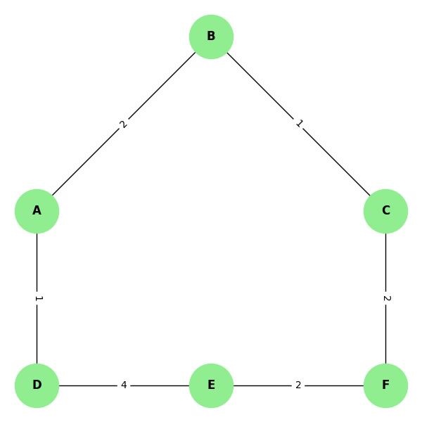
The shortest path distances between pairs of vertices, considering the weights, are as follows:

• d(A, B) = 2
• d(A, C) = 3
• d(A, D) = 1
• d(A, E) = 5
• d(A, F) = 5
• d(B, C) = 1
• d(B, D) = 3
• d(B, E) = 5
• d(B, F) = 3
• d(C, D) = 4
• d(C, E) = 4
• d(C, F) = 2
• d(D, E) = 4
• d(D, F) = 6
• d(E, F) = 2

The diameter of this graph is 6, which is the longest shortest path between vertices D and F.

Properties of Graph Diameter

The diameter of a graph has various important properties, they are −

• Unique for Connected Graphs: The diameter is well-defined and unique for connected graphs. For disconnected graphs, the diameter is considered infinite.
• Symmetric: The diameter is symmetric, meaning diam(G) is the same regardless of the direction of the edges in undirected graphs.
• Affected by Graph Changes: Adding or removing edges or vertices can change the diameter of the graph.

Diameter in Different Types of Graphs

The diameter can vary significantly depending on the type and structure of the graph −

Tree Graphs

In tree graphs, which are acyclic connected graphs, the diameter is the longest path between any two leaves (vertices with degree 1).

For example, in a binary tree, the diameter can be found by identifying the longest path between any two leaf nodes.

Complete Graphs

In complete graphs, where every pair of vertices is connected by an edge, the diameter is always 1. This is because the shortest path between any two vertices is a direct edge.

For instance, in a complete graph with n vertices, each vertex is connected to every other vertex, resulting in a diameter of 1.

Cycle Graphs

In cycle graphs, where vertices form a single cycle, the diameter is n/2 for an even number of vertices and ⌊n/2⌋ (the greatest integer less than or equal to n/2) for an odd number of vertices. This is because the longest shortest path is half the length of the cycle.

For example, in a cycle graph with 6 vertices, the diameter is 3.

Grid Graphs

In grid graphs, which are a regular lattice of vertices, the diameter depends on the dimensions of the grid. For a m x n grid graph, the diameter is m + n - 2 if m and n are the grid dimensions.

For example, in a 3 x 3 grid graph, the diameter is 4.

Diameter in Real-World Networks

Graph diameter is an important measure in various real-world networks −

Social Networks

In social networks, the diameter indicates the maximum degree of separation between individuals. It reflects the "small world" phenomenon, where most individuals are connected by a short path of acquaintances.

For example, studies on social networks like Facebook and Twitter have shown that the diameter is relatively small, indicating a high level of connectivity.

Transportation Networks

In transportation networks, the diameter represents the longest shortest path between any two locations.

For instance, in a road network, the diameter indicates the longest travel distance between any two points, helping in planning and optimizing routes.

Communication Networks

In communication networks, such as the internet, the diameter indicates the maximum number of hops (intermediate nodes) required to transmit data between any two devices. A smaller diameter signifies a more efficient network.

For example, in a well-connected communication network, the diameter is minimized to ensure faster data transmission.

Impact of Graph Modifications on Diameter

Modifying a graph by adding or removing vertices or edges can affect its diameter −

Adding Edges

Adding edges to a graph can potentially decrease its diameter by creating shorter paths between vertices. This is particularly true for sparse graphs where additional edges improve connectivity.

For example, adding an edge between two distant vertices in a tree graph can significantly reduce the diameter.

Removing Edges

Removing edges from a graph can increase its diameter by eliminating direct paths and forcing traversal through longer paths. This effect is stronger in graphs with important edges that are part of the shortest paths between many pairs of vertices.

For instance, removing an edge that connects two clusters in a graph can drastically increase the diameter.

Adding Vertices

Adding vertices to a graph does not directly affect the diameter unless new edges are added as well. The impact on the diameter depends on the placement of the new vertices and the edges connecting them.

For example, adding a vertex with edges connecting to multiple existing vertices can reduce the diameter by providing new shortcuts.

Removing Vertices

Removing vertices from a graph can increase the diameter by eliminating potential shortcuts and forcing traversal through longer paths. The impact is greater if the removed vertices are central to the graph's connectivity.

For instance, removing a central hub vertex in a star graph can significantly increase the diameter.

Diameter in Directed Graphs

In directed graphs, the diameter is calculated considering the direction of edges. The diameter is the longest shortest path considering the directed nature of the paths.

Strongly Connected Components

In strongly connected directed graphs, where every vertex is reachable from every other vertex, the diameter is well-defined. The calculation involves finding the longest shortest path considering the direction of edges.

For example, in a strongly connected component of a directed graph, the diameter reflects the longest shortest path in the directed subgraph.

Weakly Connected Components

In weakly connected directed graphs, where replacing all directed edges with undirected edges results in a connected graph, the diameter is considered infinite if there exists a pair of vertices with no directed path between them.

For instance, in a weakly connected directed graph, the diameter is infinite if there are pairs of vertices with no directed paths connecting them.