- Automata Theory - Applications
- Automata Terminology
- Basics of String in Automata
- Set Theory for Automata
- Finite Sets and Infinite Sets
- Algebraic Operations on Sets
- Relations Sets in Automata Theory
- Graph and Tree in Automata Theory
- Transition Table in Automata
- What is Queue Automata?
- Compound Finite Automata
- Complementation Process in DFA
- Closure Properties in Automata
- Concatenation Process in DFA
- Language and Grammars
- Language and Grammar
- Grammars in Theory of Computation
- Language Generated by a Grammar
- Chomsky Classification of Grammars
- Context-Sensitive Languages
- Finite Automata
- What is Finite Automata?
- Finite Automata Types
- Applications of Finite Automata
- Limitations of Finite Automata
- Two-way Deterministic Finite Automata
- Deterministic Finite Automaton (DFA)
- Non-deterministic Finite Automaton (NFA)
- NDFA to DFA Conversion
- Equivalence of NFA and DFA
- Dead State in Finite Automata
- Minimization of DFA
- Automata Moore Machine
- Automata Mealy Machine
- Moore vs Mealy Machines
- Moore to Mealy Machine
- Mealy to Moore Machine
- Myhill–Nerode Theorem
- Mealy Machine for 1’s Complement
- Finite Automata Exercises
- Complement of DFA
- Regular Expressions
- Regular Expression in Automata
- Regular Expression Identities
- Applications of Regular Expression
- Regular Expressions vs Regular Grammar
- Kleene Closure in Automata
- Arden’s Theorem in Automata
- Convert Regular Expression to Finite Automata
- Conversion of Regular Expression to DFA
- Equivalence of Two Finite Automata
- Equivalence of Two Regular Expressions
- Convert Regular Expression to Regular Grammar
- Convert Regular Grammar to Finite Automata
- Pumping Lemma in Theory of Computation
- Pumping Lemma for Regular Grammar
- Pumping Lemma for Regular Expression
- Pumping Lemma for Regular Languages
- Applications of Pumping Lemma
- Closure Properties of Regular Set
- Closure Properties of Regular Language
- Decision Problems for Regular Languages
- Decision Problems for Automata and Grammars
- Conversion of Epsilon-NFA to DFA
- Regular Sets in Theory of Computation
- Context-Free Grammars
- Context-Free Grammars (CFG)
- Derivation Tree
- Parse Tree
- Ambiguity in Context-Free Grammar
- CFG vs Regular Grammar
- Applications of Context-Free Grammar
- Left Recursion and Left Factoring
- Closure Properties of Context Free Languages
- Simplifying Context Free Grammars
- Removal of Useless Symbols in CFG
- Removal Unit Production in CFG
- Removal of Null Productions in CFG
- Linear Grammar
- Chomsky Normal Form (CNF)
- Greibach Normal Form (GNF)
- Pumping Lemma for Context-Free Grammars
- Decision Problems of CFG
- Pushdown Automata
- Pushdown Automata (PDA)
- Pushdown Automata Acceptance
- Deterministic Pushdown Automata
- Non-deterministic Pushdown Automata
- Construction of PDA from CFG
- CFG Equivalent to PDA Conversion
- Pushdown Automata Graphical Notation
- Pushdown Automata and Parsing
- Two-stack Pushdown Automata
- Turing Machines
- Basics of Turing Machine (TM)
- Representation of Turing Machine
- Examples of Turing Machine
- Turing Machine Accepted Languages
- Variations of Turing Machine
- Multi-tape Turing Machine
- Multi-head Turing Machine
- Multitrack Turing Machine
- Non-Deterministic Turing Machine
- Semi-Infinite Tape Turing Machine
- K-dimensional Turing Machine
- Enumerator Turing Machine
- Universal Turing Machine
- Restricted Turing Machine
- Convert Regular Expression to Turing Machine
- Two-stack PDA and Turing Machine
- Turing Machine as Integer Function
- Post–Turing Machine
- Turing Machine for Addition
- Turing Machine for Copying Data
- Turing Machine as Comparator
- Turing Machine for Multiplication
- Turing Machine for Subtraction
- Modifications to Standard Turing Machine
- Linear-Bounded Automata (LBA)
- Church's Thesis for Turing Machine
- Recursively Enumerable Language
- Computability & Undecidability
- Turing Language Decidability
- Undecidable Languages
- Turing Machine and Grammar
- Kuroda Normal Form
- Converting Grammar to Kuroda Normal Form
- Decidability
- Undecidability
- Reducibility
- Halting Problem
- Turing Machine Halting Problem
- Rice's Theorem in Theory of Computation
- Post’s Correspondence Problem (PCP)
- Types of Functions
- Recursive Functions
- Injective Functions
- Surjective Function
- Bijective Function
- Partial Recursive Function
- Total Recursive Function
- Primitive Recursive Function
- μ Recursive Function
- Ackermann’s Function
- Russell’s Paradox
- Gödel Numbering
- Recursive Enumerations
- Kleene's Theorem
- Kleene's Recursion Theorem
- Advanced Concepts
- Matrix Grammars
- Probabilistic Finite Automata
- Cellular Automata
- Reduction of CFG
- Reduction Theorem
- Regular expression to ∈-NFA
- Quotient Operation
- Parikh’s Theorem
- Ladner’s Theorem
What is Finite Automata?
Finite Automata, is a fundamental concept in computer science and automata theory. We get the term "automaton" from the word "automatic". In this chapter, we will explain the concept of finite automata as an overview, and its representation through a 5-tuple, and illustrate these ideas with a practical example involving a lift system.
Formal Definition of Finite Automata
A finite automata is an abstract machine used to model computation. It consists of a finite number of states and operates on input symbols to transition between these states based on a set of rules.
To represent the finite automata, we need 5 tuples −
$$\mathrm{M \:=\: (Q,\: \Sigma,\: \delta,\: q0,\: F)}$$
where −
- Q − A finite, non-empty set of states.
- Σ − A finite, non-empty set of input alphabets (symbols).
- δ − The transition function, which maps into .
- q0 − The initial state, which is an element of .
- F − A subset of representing the set of final states.
Components of 5-Tuple
Following are the components of the 5-Tuple −
- States (Q) − Q is a finite, non-empty set of states. Each state represents a unique condition or configuration of the system.
- Input Alphabets (Σ) − Σ is the finite, non-empty set of input symbols that the automaton reads to determine state transitions.
- Transition Function (δ) − δ is a set of functions that defines how the automaton transitions from one state to another based on the current state and input symbol. It can be expressed as: δ:Q×Σ→Q.
- Initial State (q0) − q0 is the initial state from which the automaton starts its computation. It belongs to the set.
- Final States (F) − F is a subset of containing one or more final states. These states signify the acceptance of the input string by the automaton.
Example of Involving an Elevator System with Three Floors
To better understand finite automata, let's consider a simple example involving a lift (elevator) system with three floors: Ground floor, First floor, and Second floor.
The lift can move between these floors based on user input. To design the automata, we need to first define the states, then the alphabets, transition, initial, state and the final state. Let's discuss each of them one by one −
- States (Q):
- Q0: Ground floor
- Q1: First floor
- Q2: Second floor
- Input Alphabets (Σ):
- 0: Go to the ground floor
- 1: Go to the first floor
- 2: Go to the second floor
- Transition System − The transition system of the lift can be represented as a directed graph.

In this directed graph, circles denote states (Q0, 1, Q2). Directed edges represent transitions based on input symbols.
The transition system of the lift can be visualized as the above mentioned directed graph with three states: Q0 (ground floor), Q1 (first floor), and Q2 (second floor).
Each state is represented by a circle. The initial state, Q0, is indicated by an inward arrow. Transitions between states are depicted by directed edges based on input symbols.
- From 0, an input of 0 leads to Q0 (self-loop), an input of 1 leads to Q1, and an input of 2 leads to Q2.
- From 1, an input of 0 transitions to Q0, an input of 1 remains in Q1 (self-loop), and an input of 2 transitions to Q2.
- From 2, an input of 0 transitions to Q0, an input of 1 transitions to Q1, and an input of 2 remains in Q2 (self-loop).
- The final state, 2, is represented by a double circle.
Transition Diagram
It is a directed graph associated with the vertices of the graph corresponding to the state of finite automata.
An example of transition diagram is given below −
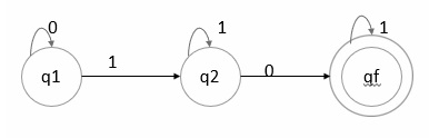
Here,
- {0,1}: Inputs
- q1: Initial state
- q2: Intermediate state
- qf: Final state
Transition Table
We can also write the same through a transition table −
| Present State | Input | Next State |
|---|---|---|
| Q0 | 0 | Q0 |
| Q0 | 1 | Q1 |
| Q0 | 2 | Q2 |
| Q1 | 0 | Q0 |
| Q1 | 1 | Q1 |
| Q1 | 2 | Q2 |
| Q2 | 0 | Q0 |
| Q2 | 1 | Q1 |
| Q2 | 2 | Q2 |
Conclusion
Finite automaton is a powerful concept used to model and analyze computational processes. By understanding the 5-tuple representation and applying it to practical examples like the lift system, we can get the basics of finite automata and understand how these abstract machines operate.
