- Automata Theory - Applications
- Automata Terminology
- Basics of String in Automata
- Set Theory for Automata
- Finite Sets and Infinite Sets
- Algebraic Operations on Sets
- Relations Sets in Automata Theory
- Graph and Tree in Automata Theory
- Transition Table in Automata
- What is Queue Automata?
- Compound Finite Automata
- Complementation Process in DFA
- Closure Properties in Automata
- Concatenation Process in DFA
- Language and Grammars
- Language and Grammar
- Grammars in Theory of Computation
- Language Generated by a Grammar
- Chomsky Classification of Grammars
- Context-Sensitive Languages
- Finite Automata
- What is Finite Automata?
- Finite Automata Types
- Applications of Finite Automata
- Limitations of Finite Automata
- Two-way Deterministic Finite Automata
- Deterministic Finite Automaton (DFA)
- Non-deterministic Finite Automaton (NFA)
- NDFA to DFA Conversion
- Equivalence of NFA and DFA
- Dead State in Finite Automata
- Minimization of DFA
- Automata Moore Machine
- Automata Mealy Machine
- Moore vs Mealy Machines
- Moore to Mealy Machine
- Mealy to Moore Machine
- Myhill–Nerode Theorem
- Mealy Machine for 1’s Complement
- Finite Automata Exercises
- Complement of DFA
- Regular Expressions
- Regular Expression in Automata
- Regular Expression Identities
- Applications of Regular Expression
- Regular Expressions vs Regular Grammar
- Kleene Closure in Automata
- Arden’s Theorem in Automata
- Convert Regular Expression to Finite Automata
- Conversion of Regular Expression to DFA
- Equivalence of Two Finite Automata
- Equivalence of Two Regular Expressions
- Convert Regular Expression to Regular Grammar
- Convert Regular Grammar to Finite Automata
- Pumping Lemma in Theory of Computation
- Pumping Lemma for Regular Grammar
- Pumping Lemma for Regular Expression
- Pumping Lemma for Regular Languages
- Applications of Pumping Lemma
- Closure Properties of Regular Set
- Closure Properties of Regular Language
- Decision Problems for Regular Languages
- Decision Problems for Automata and Grammars
- Conversion of Epsilon-NFA to DFA
- Regular Sets in Theory of Computation
- Context-Free Grammars
- Context-Free Grammars (CFG)
- Derivation Tree
- Parse Tree
- Ambiguity in Context-Free Grammar
- CFG vs Regular Grammar
- Applications of Context-Free Grammar
- Left Recursion and Left Factoring
- Closure Properties of Context Free Languages
- Simplifying Context Free Grammars
- Removal of Useless Symbols in CFG
- Removal Unit Production in CFG
- Removal of Null Productions in CFG
- Linear Grammar
- Chomsky Normal Form (CNF)
- Greibach Normal Form (GNF)
- Pumping Lemma for Context-Free Grammars
- Decision Problems of CFG
- Pushdown Automata
- Pushdown Automata (PDA)
- Pushdown Automata Acceptance
- Deterministic Pushdown Automata
- Non-deterministic Pushdown Automata
- Construction of PDA from CFG
- CFG Equivalent to PDA Conversion
- Pushdown Automata Graphical Notation
- Pushdown Automata and Parsing
- Two-stack Pushdown Automata
- Turing Machines
- Basics of Turing Machine (TM)
- Representation of Turing Machine
- Examples of Turing Machine
- Turing Machine Accepted Languages
- Variations of Turing Machine
- Multi-tape Turing Machine
- Multi-head Turing Machine
- Multitrack Turing Machine
- Non-Deterministic Turing Machine
- Semi-Infinite Tape Turing Machine
- K-dimensional Turing Machine
- Enumerator Turing Machine
- Universal Turing Machine
- Restricted Turing Machine
- Convert Regular Expression to Turing Machine
- Two-stack PDA and Turing Machine
- Turing Machine as Integer Function
- Post–Turing Machine
- Turing Machine for Addition
- Turing Machine for Copying Data
- Turing Machine as Comparator
- Turing Machine for Multiplication
- Turing Machine for Subtraction
- Modifications to Standard Turing Machine
- Linear-Bounded Automata (LBA)
- Church's Thesis for Turing Machine
- Recursively Enumerable Language
- Computability & Undecidability
- Turing Language Decidability
- Undecidable Languages
- Turing Machine and Grammar
- Kuroda Normal Form
- Converting Grammar to Kuroda Normal Form
- Decidability
- Undecidability
- Reducibility
- Halting Problem
- Turing Machine Halting Problem
- Rice's Theorem in Theory of Computation
- Post’s Correspondence Problem (PCP)
- Types of Functions
- Recursive Functions
- Injective Functions
- Surjective Function
- Bijective Function
- Partial Recursive Function
- Total Recursive Function
- Primitive Recursive Function
- μ Recursive Function
- Ackermann’s Function
- Russell’s Paradox
- Gödel Numbering
- Recursive Enumerations
- Kleene's Theorem
- Kleene's Recursion Theorem
- Advanced Concepts
- Matrix Grammars
- Probabilistic Finite Automata
- Cellular Automata
- Reduction of CFG
- Reduction Theorem
- Regular expression to ∈-NFA
- Quotient Operation
- Parikh’s Theorem
- Ladner’s Theorem
Moore and Mealy Machines
Finite automata may have outputs corresponding to each transition. There are two types of finite state machines that generate output −
- Mealy Machine
- Moore machine
Mealy Machine
A Mealy Machine is an FSM whose output depends on the present state as well as the present input.
It can be described by a 6 tuple (Q, ∑, O, δ, X, q0) where −
Q is a finite set of states.
∑ is a finite set of symbols called the input alphabet.
O is a finite set of symbols called the output alphabet.
δ is the input transition function where δ: Q × ∑ → Q
X is the output transition function where X: Q × ∑ → O
q0 is the initial state from where any input is processed (q0 ∈ Q).
The state table of a Mealy Machine is shown below −
| Present state | Next state | |||
|---|---|---|---|---|
| input = 0 | input = 1 | |||
| State | Output | State | Output | |
| → a | b | x1 | c | x1 |
| b | b | x2 | d | x3 |
| c | d | x3 | c | x1 |
| d | d | x3 | d | x2 |
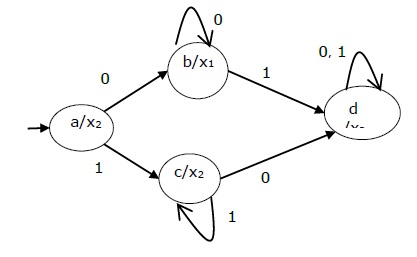
The state diagram of the above Mealy Machine is −
Moore Machine
Moore machine is an FSM whose outputs depend on only the present state.
A Moore machine can be described by a 6 tuple (Q, ∑, O, δ, X, q0) where −
Q is a finite set of states.
∑ is a finite set of symbols called the input alphabet.
O is a finite set of symbols called the output alphabet.
δ is the input transition function where δ: Q × ∑ → Q
X is the output transition function where X: Q → O
q0 is the initial state from where any input is processed (q0 ∈ Q).
The state table of a Moore Machine is shown below −
| Present state | Next State | Output | |
|---|---|---|---|
| Input = 0 | Input = 1 | ||
| → a | b | c | x2 |
| b | b | d | x1 |
| c | c | d | x2 |
| d | d | d | x3 |
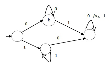
The state diagram of the above Moore Machine is −
Mealy Machine vs. Moore Machine
The following table highlights the points that differentiate a Mealy Machine from a Moore Machine.
| Mealy Machine | Moore Machine |
|---|---|
| Output depends both upon the present state and the present input | Output depends only upon the present state. |
| Generally, it has fewer states than Moore Machine. | Generally, it has more states than Mealy Machine. |
| The value of the output function is a function of the transitions and the changes, when the input logic on the present state is done. | The value of the output function is a function of the current state and the changes at the clock edges, whenever state changes occur. |
| Mealy machines react faster to inputs. They generally react in the same clock cycle. | In Moore machines, more logic is required to decode the outputs resulting in more circuit delays. They generally react one clock cycle later. |
Moore Machine to Mealy Machine
Algorithm 4
Input − Moore Machine
Output − Mealy Machine
Step 1 − Take a blank Mealy Machine transition table format.
Step 2 − Copy all the Moore Machine transition states into this table format.
Step 3 − Check the present states and their corresponding outputs in the Moore Machine state table; if for a state Qi output is m, copy it into the output columns of the Mealy Machine state table wherever Qi appears in the next state.
Example
Let us consider the following Moore machine −
| Present State | Next State | Output | |
|---|---|---|---|
| a = 0 | a = 1 | ||
| → a | d | b | 1 |
| b | a | d | 0 |
| c | c | c | 0 |
| d | b | a | 1 |
Now we apply Algorithm 4 to convert it to Mealy Machine.
Step 1 & 2 −
| Present State | Next State | |||
|---|---|---|---|---|
| a = 0 | a = 1 | |||
| State | Output | State | Output | |
| → a | d | b | ||
| b | a | d | ||
| c | c | c | ||
| d | b | a | ||
Step 3 −
| Present State | Next State | |||
|---|---|---|---|---|
| a = 0 | a = 1 | |||
| State | Output | State | Output | |
| => a | d | 1 | b | 0 |
| b | a | 1 | d | 1 |
| c | c | 0 | c | 0 |
| d | b | 0 | a | 1 |
Mealy Machine to Moore Machine
Algorithm 5
Input − Mealy Machine
Output − Moore Machine
Step 1 − Calculate the number of different outputs for each state (Qi) that are available in the state table of the Mealy machine.
Step 2 − If all the outputs of Qi are same, copy state Qi. If it has n distinct outputs, break Qi into n states as Qin where n = 0, 1, 2.......
Step 3 − If the output of the initial state is 1, insert a new initial state at the beginning which gives 0 output.
Example
Let us consider the following Mealy Machine −
| Present State | Next State | |||
|---|---|---|---|---|
| a = 0 | a = 1 | |||
| Next State | Output | Next State | Output | |
| → a | d | 0 | b | 1 |
| b | a | 1 | d | 0 |
| c | c | 1 | c | 0 |
| d | b | 0 | a | 1 |
Here, states a and d give only 1 and 0 outputs respectively, so we retain states a and d. But states b and c produce different outputs (1 and 0). So, we divide b into b0, b1 and c into c0, c1.
| Present State | Next State | Output | |
|---|---|---|---|
| a = 0 | a = 1 | ||
| → a | d | b1 | 1 |
| b0 | a | d | 0 |
| b1 | a | d | 1 |
| c0 | c1 | C0 | 0 |
| c1 | c1 | C0 | 1 |
| d | b0 | a | 0 |
