- Automata Theory - Applications
- Automata Terminology
- Basics of String in Automata
- Set Theory for Automata
- Finite Sets and Infinite Sets
- Algebraic Operations on Sets
- Relations Sets in Automata Theory
- Graph and Tree in Automata Theory
- Transition Table in Automata
- What is Queue Automata?
- Compound Finite Automata
- Complementation Process in DFA
- Closure Properties in Automata
- Concatenation Process in DFA
- Language and Grammars
- Language and Grammar
- Grammars in Theory of Computation
- Language Generated by a Grammar
- Chomsky Classification of Grammars
- Context-Sensitive Languages
- Finite Automata
- What is Finite Automata?
- Finite Automata Types
- Applications of Finite Automata
- Limitations of Finite Automata
- Two-way Deterministic Finite Automata
- Deterministic Finite Automaton (DFA)
- Non-deterministic Finite Automaton (NFA)
- NDFA to DFA Conversion
- Equivalence of NFA and DFA
- Dead State in Finite Automata
- Minimization of DFA
- Automata Moore Machine
- Automata Mealy Machine
- Moore vs Mealy Machines
- Moore to Mealy Machine
- Mealy to Moore Machine
- Myhill–Nerode Theorem
- Mealy Machine for 1’s Complement
- Finite Automata Exercises
- Complement of DFA
- Regular Expressions
- Regular Expression in Automata
- Regular Expression Identities
- Applications of Regular Expression
- Regular Expressions vs Regular Grammar
- Kleene Closure in Automata
- Arden’s Theorem in Automata
- Convert Regular Expression to Finite Automata
- Conversion of Regular Expression to DFA
- Equivalence of Two Finite Automata
- Equivalence of Two Regular Expressions
- Convert Regular Expression to Regular Grammar
- Convert Regular Grammar to Finite Automata
- Pumping Lemma in Theory of Computation
- Pumping Lemma for Regular Grammar
- Pumping Lemma for Regular Expression
- Pumping Lemma for Regular Languages
- Applications of Pumping Lemma
- Closure Properties of Regular Set
- Closure Properties of Regular Language
- Decision Problems for Regular Languages
- Decision Problems for Automata and Grammars
- Conversion of Epsilon-NFA to DFA
- Regular Sets in Theory of Computation
- Context-Free Grammars
- Context-Free Grammars (CFG)
- Derivation Tree
- Parse Tree
- Ambiguity in Context-Free Grammar
- CFG vs Regular Grammar
- Applications of Context-Free Grammar
- Left Recursion and Left Factoring
- Closure Properties of Context Free Languages
- Simplifying Context Free Grammars
- Removal of Useless Symbols in CFG
- Removal Unit Production in CFG
- Removal of Null Productions in CFG
- Linear Grammar
- Chomsky Normal Form (CNF)
- Greibach Normal Form (GNF)
- Pumping Lemma for Context-Free Grammars
- Decision Problems of CFG
- Pushdown Automata
- Pushdown Automata (PDA)
- Pushdown Automata Acceptance
- Deterministic Pushdown Automata
- Non-deterministic Pushdown Automata
- Construction of PDA from CFG
- CFG Equivalent to PDA Conversion
- Pushdown Automata Graphical Notation
- Pushdown Automata and Parsing
- Two-stack Pushdown Automata
- Turing Machines
- Basics of Turing Machine (TM)
- Representation of Turing Machine
- Examples of Turing Machine
- Turing Machine Accepted Languages
- Variations of Turing Machine
- Multi-tape Turing Machine
- Multi-head Turing Machine
- Multitrack Turing Machine
- Non-Deterministic Turing Machine
- Semi-Infinite Tape Turing Machine
- K-dimensional Turing Machine
- Enumerator Turing Machine
- Universal Turing Machine
- Restricted Turing Machine
- Convert Regular Expression to Turing Machine
- Two-stack PDA and Turing Machine
- Turing Machine as Integer Function
- Post–Turing Machine
- Turing Machine for Addition
- Turing Machine for Copying Data
- Turing Machine as Comparator
- Turing Machine for Multiplication
- Turing Machine for Subtraction
- Modifications to Standard Turing Machine
- Linear-Bounded Automata (LBA)
- Church's Thesis for Turing Machine
- Recursively Enumerable Language
- Computability & Undecidability
- Turing Language Decidability
- Undecidable Languages
- Turing Machine and Grammar
- Kuroda Normal Form
- Converting Grammar to Kuroda Normal Form
- Decidability
- Undecidability
- Reducibility
- Halting Problem
- Turing Machine Halting Problem
- Rice's Theorem in Theory of Computation
- Post’s Correspondence Problem (PCP)
- Types of Functions
- Recursive Functions
- Injective Functions
- Surjective Function
- Bijective Function
- Partial Recursive Function
- Total Recursive Function
- Primitive Recursive Function
- μ Recursive Function
- Ackermann’s Function
- Russell’s Paradox
- Gödel Numbering
- Recursive Enumerations
- Kleene's Theorem
- Kleene's Recursion Theorem
- Advanced Concepts
- Matrix Grammars
- Probabilistic Finite Automata
- Cellular Automata
- Reduction of CFG
- Reduction Theorem
- Regular expression to ∈-NFA
- Quotient Operation
- Parikh’s Theorem
- Ladner’s Theorem
Two-Way Deterministic Finite Automata
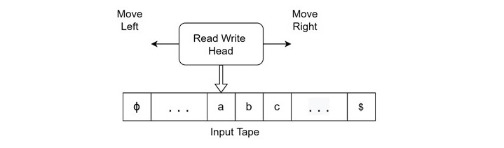
There is a variation of finite automata which is known as two-way deterministic finite automata or 2DFA. This is an extension of the deterministic finite automata (DFA). Unlike the DFA, which only allows the reading head to move in right direction only, a 2DFA allows movement in both directions (both left and right).
A 2DFA provides more flexibility in recognizing patterns in input strings. In this chapter, we will explain the concept of 2DFA and its components, functionality, and the acceptance and rejection conditions, with some examples.
Components of a 2DFA
A two-way finite automata can also be defined through a quintuple M = (Q,Σ,δ,Q0,F) where −
- Q is the set of states
- Σ is the input alphabet
- Q0 is the initial state
- F is the set of final states
- δ is the transition function
But in the transition function, it is different. For a DFA, the transition function δ maps Q × Σ to Q.
In the case of a 2DFA, the transition function δ maps Q × Σ to Q{L,R}, where L stands for a left move and R for a right move.
The Operations of 2DFA
Like DFA, the 2DFA also starts at the leftmost symbol of the input string in the initial state 0. Depending on the current state and the symbol read, it transitions to a new state and moves the reading head either left or right. We can understand it further through the configuration.
Configuration for 2DFA
Consider an input string w = a1 a2 … an If the automaton is in state Q and reads symbol ai −
- The current configuration can be described as w = a1 a2 … a(i-1) Qai a(i+1) … an.
- If δ(Q,ai ) = (P,R), where the next state will be P, and the head will move to the right.
- If δ(Q,ai ) = (P,L), where the next state will be P, and the head will move to the left.
Acceptance and Rejection Conditions
After the configuration, we must understand the acceptance and rejection of the machine. Let us understand them one by one.
An input is accepted when, all symbols are processed, and the automaton moves off the right end of the tape while in a final state.
An input can be rejected in three ways −
- Moving off the right end of the tape in a non-final state
- Moving off the left end of the tape
- Entering a loop (Repeatedly revisiting the same configuration without making progress)
Instantaneous Description (ID)
To track the working of 2DFA, we must know the instantaneous description (ID) for 2DFA. These are nothing but the snapshot of its current state, the remaining input, and the position of the reading head.
It can be denoted as a string in Σ* QΣ*. Let us understand one example ID
For an input string w = a1 a2…an and current state Q reading ai, the ID is,
$$\mathrm{a_{1} \:a_{2}\: \dotso\: a_{(i-1)} \: Qa_{i} \: a_{(i+1)}\:\dotso\: a_{n}}$$
If δ(Q,ai ) = (P,R), the head moves right, and the new ID is a1 a2 … a(i-1) ai Pa(i+1) … an.
Language Accepted by a 2DFA
After knowing the basics, let us now understand which language can be accepted by 2DFA.
The language accepted by a 2DFA is M = (Q, Σ, δ, Q0, F) the set of strings w such that starting from the initial state Q0, the w can be processed and the automaton reaches a final state in F.
This can be defined formally like −
L(M) = { w ∈ Σ* | starting in Q0, w leads to some Qf ∈ F in finite steps}
Sample 2DFA Example
So far, we have seen some theoretical concepts. Let's understand a sample 2DFA with its definition and transition in action.
Consider the following 2DFA, M −
- States: Q = { Q0, Q1, Q2, Q3 }
- Input alphabet: Σ = { a,b }
- Initial state: Q0
- Final state: F = { Q2 }
Transition Table
Its transition table will be like the one shown here −
| Present State | Input | Next State | Direction |
|---|---|---|---|
| Q0 | a | Q1 | Right |
| Q0 | b | Q1 | Left |
| Q1 | a | Q0 | Left |
| Q1 | b | Q3 | Right |
| Q3 | a | Q1 | Left |
| Q3 | b | Q2 | Right |
| Q2 | a | Q2 | Right |
| Q2 | b | Q2 | Left |
Conclusion
In this chapter, we explained the basics of 2DFA. The 2DFA offers enhanced capabilities over a traditional Right-only DFA. It allows bidirectional movement of the reading head, which helps for more complex string processing. We explained their properties, definition, formation, and examples with the help of instantaneous description and an example with full detail.
