Post Turing Machine in Automata Theory

---

---

The Post-Turing Machine is an advanced model upon the finite automata and pushdown automata. The Post-Turing Machine uses an external memory in the form of a queue. The queue allows it to perform more complex operations. In this chapter, we will cover the basics, explain how the machine works, and walk through a detailed example for a better understanding.

What is the Post-Turing Machine?

The Post-Turing Machine is named after the Polish mathematician Emil Post. This machine is similar to the Turing machine but with a key difference: it uses a queue as its external memory. In a queue, operations are performed using two pointers: the front pointer and the rear pointer.

• Queue − We know the Queue from data structures. The queue is a linear data structure where elements are inserted at the rear and removed from the front. This structure follows the First In, First Out (FIFO) principle.
• Front Pointer − This pointer points to the first element of the queue.
• Rear Pointer − This pointer points to the last element of the queue.

In the Post-Turing Machine, the queue is used to store symbols, and operations are performed by inserting and deleting these symbols.

Definition of the Post-Turing Machine

The Post-Turing Machine is defined using seven tuples, which are as follows −

• Q − A finite set of states.
• Σ − The input alphabet.
• Γ − The queue symbols, which include all symbols in Σ and a special symbol Z0.
• δ − The transition function.
• q0 − The initial state, which is a member of Q.
• Z0 − A special symbol that marks the end of the string in the queue.
• F − The set of final states, which is a subset of Q.

The functional block diagram of the Post-Turing Machine looks like this −

Transition Function in the Post-Turing Machine

The transition function in the Post-Turing Machine defines how the machine processes input and interacts with the queue. There are two main operations −

• Delete Operation − This operation removes a symbol from the front of the queue.
• Insert Operation − This operation adds a symbol to the rear of the queue.

The transition function can be represented in several ways, depending on what action is being performed. Here are the four primary forms of the transition function −

• δ(q1, A) → (q2, B) − In this transition, the machine moves from state q1 to state q2. It deletes the symbol A from the front of the queue and inserts the symbol B at the rear.
• δ(q1, A) → (q2, ε) − Here, the machine moves from state q1 to state q2, deletes the symbol A from the front of the queue, but does not insert any new symbol at the rear.
• δ(q1, ε) → (q2, A) − In this case, the machine moves from state q1 to state q2 without deleting any symbol from the front, but it inserts the symbol A at the rear of the queue.
• δ(q1, ε) → (q2, ε) − This transition moves the machine from state q1 to state q2 without deleting any symbol from the front and without inserting any new symbol at the rear.

These transitions allow the Post-Turing Machine to manipulate the queue in different ways, depending on the needs of the computation.

Example of a Post-Turing Machine

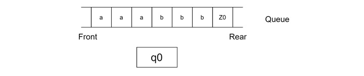
Let us see one example of this type of machine. Consider a queue containing the string L = {aⁿ bⁿ}, for example aaabbbZ0, where Z0 is the special symbol marking the end of the string.

Initial State − The post machine starts in state q0, insert string inside the queue.

Step 1

• Read the first 'a' from the input string.
• Delete the 'a' from the front of the queue (since the first occurrence of 'a' is encountered).
• Insert 'ε' (nothing) at the rear of the queue.
• Transition to state q1.

Step 2

• Read the second 'a' from the input string.
• Delete the 'a' from the front of the queue.
• Insert 'a' at the rear of the queue.
• Remain in state q1.

Step 3

• Read the third 'a' from the input string.
• Delete the 'a' from the front of the queue.
• Insert 'a' at the rear of the queue.
• Remain in state q1.

Step 4

• Read the first 'b' from the input string.
• Delete the 'b' from the front of the queue.
• Insert 'ε' (nothing) at the rear of the queue.
• Transition to state q2.

Step 5

• Read the second 'b' from the input string.
• Delete the 'b' from the front of the queue.
• Insert 'b' at the rear of the queue.
• Remain in state q2.

Step 6

• Read the third 'b' from the input string.
• Delete the 'b' from the front of the queue.
• Insert 'b' at the rear of the queue.
• Remain in state q2.

Step 7

• Read the 'Z0' from the input string.
• Delete the ' Z0' from the front of the queue.
• Insert ' Z0' at the rear of the queue.
• Remain in state q2.

Now repeat these steps. Currently after the first iteration, it is "abZ0". In the next iteration, it will be "abZ0". Thereafter, it will be only "Z0"

Transition Diagram − If we formulate this through state transition diagram, it will be look like −

Conclusion

The Post-Turing Machine is a powerful computational model that extends finite automata and pushdown automata. It uses a queue as external memory; it can perform more complex operations. In this chapter, we covered the basics of this machine with examples to explain stepbystep how a language can be detected and we also presented a state diagram for the generated machine.