- Automata Theory - Applications
- Automata Terminology
- Basics of String in Automata
- Set Theory for Automata
- Finite Sets and Infinite Sets
- Algebraic Operations on Sets
- Relations Sets in Automata Theory
- Graph and Tree in Automata Theory
- Transition Table in Automata
- What is Queue Automata?
- Compound Finite Automata
- Complementation Process in DFA
- Closure Properties in Automata
- Concatenation Process in DFA
- Language and Grammars
- Language and Grammar
- Grammars in Theory of Computation
- Language Generated by a Grammar
- Chomsky Classification of Grammars
- Context-Sensitive Languages
- Finite Automata
- What is Finite Automata?
- Finite Automata Types
- Applications of Finite Automata
- Limitations of Finite Automata
- Two-way Deterministic Finite Automata
- Deterministic Finite Automaton (DFA)
- Non-deterministic Finite Automaton (NFA)
- NDFA to DFA Conversion
- Equivalence of NFA and DFA
- Dead State in Finite Automata
- Minimization of DFA
- Automata Moore Machine
- Automata Mealy Machine
- Moore vs Mealy Machines
- Moore to Mealy Machine
- Mealy to Moore Machine
- Myhill–Nerode Theorem
- Mealy Machine for 1’s Complement
- Finite Automata Exercises
- Complement of DFA
- Regular Expressions
- Regular Expression in Automata
- Regular Expression Identities
- Applications of Regular Expression
- Regular Expressions vs Regular Grammar
- Kleene Closure in Automata
- Arden’s Theorem in Automata
- Convert Regular Expression to Finite Automata
- Conversion of Regular Expression to DFA
- Equivalence of Two Finite Automata
- Equivalence of Two Regular Expressions
- Convert Regular Expression to Regular Grammar
- Convert Regular Grammar to Finite Automata
- Pumping Lemma in Theory of Computation
- Pumping Lemma for Regular Grammar
- Pumping Lemma for Regular Expression
- Pumping Lemma for Regular Languages
- Applications of Pumping Lemma
- Closure Properties of Regular Set
- Closure Properties of Regular Language
- Decision Problems for Regular Languages
- Decision Problems for Automata and Grammars
- Conversion of Epsilon-NFA to DFA
- Regular Sets in Theory of Computation
- Context-Free Grammars
- Context-Free Grammars (CFG)
- Derivation Tree
- Parse Tree
- Ambiguity in Context-Free Grammar
- CFG vs Regular Grammar
- Applications of Context-Free Grammar
- Left Recursion and Left Factoring
- Closure Properties of Context Free Languages
- Simplifying Context Free Grammars
- Removal of Useless Symbols in CFG
- Removal Unit Production in CFG
- Removal of Null Productions in CFG
- Linear Grammar
- Chomsky Normal Form (CNF)
- Greibach Normal Form (GNF)
- Pumping Lemma for Context-Free Grammars
- Decision Problems of CFG
- Pushdown Automata
- Pushdown Automata (PDA)
- Pushdown Automata Acceptance
- Deterministic Pushdown Automata
- Non-deterministic Pushdown Automata
- Construction of PDA from CFG
- CFG Equivalent to PDA Conversion
- Pushdown Automata Graphical Notation
- Pushdown Automata and Parsing
- Two-stack Pushdown Automata
- Turing Machines
- Basics of Turing Machine (TM)
- Representation of Turing Machine
- Examples of Turing Machine
- Turing Machine Accepted Languages
- Variations of Turing Machine
- Multi-tape Turing Machine
- Multi-head Turing Machine
- Multitrack Turing Machine
- Non-Deterministic Turing Machine
- Semi-Infinite Tape Turing Machine
- K-dimensional Turing Machine
- Enumerator Turing Machine
- Universal Turing Machine
- Restricted Turing Machine
- Convert Regular Expression to Turing Machine
- Two-stack PDA and Turing Machine
- Turing Machine as Integer Function
- Post–Turing Machine
- Turing Machine for Addition
- Turing Machine for Copying Data
- Turing Machine as Comparator
- Turing Machine for Multiplication
- Turing Machine for Subtraction
- Modifications to Standard Turing Machine
- Linear-Bounded Automata (LBA)
- Church's Thesis for Turing Machine
- Recursively Enumerable Language
- Computability & Undecidability
- Turing Language Decidability
- Undecidable Languages
- Turing Machine and Grammar
- Kuroda Normal Form
- Converting Grammar to Kuroda Normal Form
- Decidability
- Undecidability
- Reducibility
- Halting Problem
- Turing Machine Halting Problem
- Rice's Theorem in Theory of Computation
- Post’s Correspondence Problem (PCP)
- Types of Functions
- Recursive Functions
- Injective Functions
- Surjective Function
- Bijective Function
- Partial Recursive Function
- Total Recursive Function
- Primitive Recursive Function
- μ Recursive Function
- Ackermann’s Function
- Russell’s Paradox
- Gödel Numbering
- Recursive Enumerations
- Kleene's Theorem
- Kleene's Recursion Theorem
- Advanced Concepts
- Matrix Grammars
- Probabilistic Finite Automata
- Cellular Automata
- Reduction of CFG
- Reduction Theorem
- Regular expression to ∈-NFA
- Quotient Operation
- Parikh’s Theorem
- Ladner’s Theorem
Algebraic Operations on Sets
In Set Theory concepts and Automata Theory, finite sets are frequently used. For example, in automata theory, we use machine descriptions for finite state machines, and other automata which are represented in tuples and each element in that tuple uses several sets which are finite in nature. But to use sets we must know some of the operations involved.
In this chapter, we will go through the arithmetic operations of set theory in detail with diagrams and examples.
Union of Two Sets
The union of two sets denotes the whole set of elements that are present in A or B or both. The union of A and B is denoted as A ∪ B. For example, A = {2, 3, 4} and B = {3, 5, 6}, A ∪ B = {2, 3, 4, 5, 6} which is nothing but {x | x ∈A or x ∈B}.
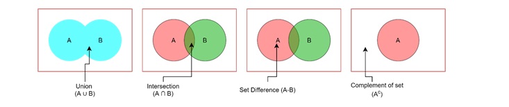
In Figure-1, the first diagram represents the union operation where blue region is covering both A and B.
Intersection of Two Sets
The intersection of two sets denotes the common set which is present in both the candidate sets. The intersection of A and B is denoted as A ∩ B. For example, A = {2, 3, 4} and B = {3, 4, 6}, A ∩ B = {3, 4} which is nothing but {x | x ∈A and x ∈B}.
In Figure-1, the second diagram represents the intersection operation where common region covered by both the sets A and B is the intersection
Set Difference
The set difference of two sets denotes the set where the common elements of two sets are missing. This is little bit complex and we can understand through examples. The set difference of B from A is denoted as A - B. For example, A = {2, 3, 4} and B = {3, 4, 6}, A - B = {2} this is the removal of A ∩ B from A. This can be represented as {x | x ∈A and x ∉ B}.
In Figure-1, the third diagram represents the set difference from A to B operation where the common region covered by both the sets A and B is the intersection and from A, we remove the intersection to get the difference.
Set Complement
The complement of a set A is the all elements which are not in A, in other words the difference of universal set and the set A is the complement. We denote complement by A’ or Ac, which is a subset of a large set U, defined by A′ = {x ∈U: x ∉ A}.
In Figure-1, the fourth diagram represents the complement of set A where common region covered by A is removed from universal set U.
Cartesian Product of Two Sets
The Cartesian product of two sets A and B is denoted as A × B. For example, A = {2, 3, 4, 5} and B = {3, 4}, A × B = {(2, 3), (2, 4), (3, 3), (3, 4),(4, 3), (4, 4), (5, 3), (5, 4)}.
Power Set
The power set of a set A is the set of all possible subsets of A, such as {a, b}, and for a set of elements n, the number of elements in the power set of A is 2n. For example, for set A = {1, 2}, the power set is {{}, {1}, {2}, {1,2}} with 22 = 4 elements.
Properties of Set Operations
The following table summarizes the properties of Set Operations −
| Property | Expression |
|---|---|
| Null Set Property | A ∪ ∅ = A, A ∩ ∅ = A |
| Universal Set Property | A ∪ U = U, A ∩ U = A (where A ⊂ U) |
| Idempotent Law | A ∪ A = A, A ∩ A = A |
| Commutative Property | A ∪ B = B ∪ A, A ∩ B = B ∩ A |
| Associative Property | A ∪ (B ∪ C) = (A ∪B) ∪ C A ∩ (B ∩ C) = (A ∩ B) ∩ C |
| Distributive Property | A ∪ (B ∩ C) = (A ∪ B) ∩ (B ∪ C), A ∩ (B ∪ C) = (A ∩ B) ∪ (B ∩ C) |
| Complement Properties | A ∪ AC = U A ∩ AC = ∅ (AC)C = A |
| De Morgan's Laws | (A ∪ B)C = AC ∩ BC, (A ∩ B)C = AC ∪ BC |
| Set Difference Properties | A − (B ∪ C) = (A − B) ∩ (A − C) A − (B ∩ C) = (A − B) ∪ (A − C) |
Conclusion
In this chapter, we explained the arithmetic operations on sets, including union, intersection, set difference, complement, Cartesian product and power set.
We also covered the possible properties of set theory which are very much useful while using sets in automata theory along with Boolean algebra.
