- Automata Theory - Applications
- Automata Terminology
- Basics of String in Automata
- Set Theory for Automata
- Finite Sets and Infinite Sets
- Algebraic Operations on Sets
- Relations Sets in Automata Theory
- Graph and Tree in Automata Theory
- Transition Table in Automata
- What is Queue Automata?
- Compound Finite Automata
- Complementation Process in DFA
- Closure Properties in Automata
- Concatenation Process in DFA
- Language and Grammars
- Language and Grammar
- Grammars in Theory of Computation
- Language Generated by a Grammar
- Chomsky Classification of Grammars
- Context-Sensitive Languages
- Finite Automata
- What is Finite Automata?
- Finite Automata Types
- Applications of Finite Automata
- Limitations of Finite Automata
- Two-way Deterministic Finite Automata
- Deterministic Finite Automaton (DFA)
- Non-deterministic Finite Automaton (NFA)
- NDFA to DFA Conversion
- Equivalence of NFA and DFA
- Dead State in Finite Automata
- Minimization of DFA
- Automata Moore Machine
- Automata Mealy Machine
- Moore vs Mealy Machines
- Moore to Mealy Machine
- Mealy to Moore Machine
- Myhill–Nerode Theorem
- Mealy Machine for 1’s Complement
- Finite Automata Exercises
- Complement of DFA
- Regular Expressions
- Regular Expression in Automata
- Regular Expression Identities
- Applications of Regular Expression
- Regular Expressions vs Regular Grammar
- Kleene Closure in Automata
- Arden’s Theorem in Automata
- Convert Regular Expression to Finite Automata
- Conversion of Regular Expression to DFA
- Equivalence of Two Finite Automata
- Equivalence of Two Regular Expressions
- Convert Regular Expression to Regular Grammar
- Convert Regular Grammar to Finite Automata
- Pumping Lemma in Theory of Computation
- Pumping Lemma for Regular Grammar
- Pumping Lemma for Regular Expression
- Pumping Lemma for Regular Languages
- Applications of Pumping Lemma
- Closure Properties of Regular Set
- Closure Properties of Regular Language
- Decision Problems for Regular Languages
- Decision Problems for Automata and Grammars
- Conversion of Epsilon-NFA to DFA
- Regular Sets in Theory of Computation
- Context-Free Grammars
- Context-Free Grammars (CFG)
- Derivation Tree
- Parse Tree
- Ambiguity in Context-Free Grammar
- CFG vs Regular Grammar
- Applications of Context-Free Grammar
- Left Recursion and Left Factoring
- Closure Properties of Context Free Languages
- Simplifying Context Free Grammars
- Removal of Useless Symbols in CFG
- Removal Unit Production in CFG
- Removal of Null Productions in CFG
- Linear Grammar
- Chomsky Normal Form (CNF)
- Greibach Normal Form (GNF)
- Pumping Lemma for Context-Free Grammars
- Decision Problems of CFG
- Pushdown Automata
- Pushdown Automata (PDA)
- Pushdown Automata Acceptance
- Deterministic Pushdown Automata
- Non-deterministic Pushdown Automata
- Construction of PDA from CFG
- CFG Equivalent to PDA Conversion
- Pushdown Automata Graphical Notation
- Pushdown Automata and Parsing
- Two-stack Pushdown Automata
- Turing Machines
- Basics of Turing Machine (TM)
- Representation of Turing Machine
- Examples of Turing Machine
- Turing Machine Accepted Languages
- Variations of Turing Machine
- Multi-tape Turing Machine
- Multi-head Turing Machine
- Multitrack Turing Machine
- Non-Deterministic Turing Machine
- Semi-Infinite Tape Turing Machine
- K-dimensional Turing Machine
- Enumerator Turing Machine
- Universal Turing Machine
- Restricted Turing Machine
- Convert Regular Expression to Turing Machine
- Two-stack PDA and Turing Machine
- Turing Machine as Integer Function
- Post–Turing Machine
- Turing Machine for Addition
- Turing Machine for Copying Data
- Turing Machine as Comparator
- Turing Machine for Multiplication
- Turing Machine for Subtraction
- Modifications to Standard Turing Machine
- Linear-Bounded Automata (LBA)
- Church's Thesis for Turing Machine
- Recursively Enumerable Language
- Computability & Undecidability
- Turing Language Decidability
- Undecidable Languages
- Turing Machine and Grammar
- Kuroda Normal Form
- Converting Grammar to Kuroda Normal Form
- Decidability
- Undecidability
- Reducibility
- Halting Problem
- Turing Machine Halting Problem
- Rice's Theorem in Theory of Computation
- Post’s Correspondence Problem (PCP)
- Types of Functions
- Recursive Functions
- Injective Functions
- Surjective Function
- Bijective Function
- Partial Recursive Function
- Total Recursive Function
- Primitive Recursive Function
- μ Recursive Function
- Ackermann’s Function
- Russell’s Paradox
- Gödel Numbering
- Recursive Enumerations
- Kleene's Theorem
- Kleene's Recursion Theorem
- Advanced Concepts
- Matrix Grammars
- Probabilistic Finite Automata
- Cellular Automata
- Reduction of CFG
- Reduction Theorem
- Regular expression to ∈-NFA
- Quotient Operation
- Parikh’s Theorem
- Ladner’s Theorem
Moore Machine in Automata Theory
In the finite automata domain, unlike NFA or DFA, there are other machines that can produce outputs when inputs are consumed. One such machine is Moore Machine. In this chapter, we will explain the concept of Moore Machine, then the components and strategy to form a Moore machine by using transition graph for a better understanding.
The Concept of Moore Machine
In finite automata theory, the Moore machine is a type of machine that can produce output. Another variation of output producing machine is Mealy machine on which will discuss on the next article. Unlike finite automata we have studied before, such as NFA and DFA, a Moore machines' output capability is the unique thing. In the Moore machine's output depends solely on the present state. This is important to understand how Moore Machines operate and how they are constructed.
We can use NFA or DFA, where we normally assess whether a string is accepted or rejected by starting from an initial state and perhaps reaching several end states. A final state is not necessary for Moore machines. It just has a beginning state. Rather, the Moore machine generates an output when we reach at any state for each input that is provided to it.
Components of a Moore Machine
Moore machines are six-tuples by their definitions. which are similar to those we learnt in NFA and DFA but with one additional component.
Let's define these tuples −
- Q − A finite set of states (e.g., Q0, Q1, Q2).
- Σ (Sigma) − A finite set called the input alphabet (e.g., A, B).
- δ (Small delta) − The transition function, where Q × Σ → Q. It describes the state transitions based on the input alphabet.
- q0 − The initial state.
- O − A finite set of symbols called the output alphabet.
- λ (Lambda) − The output transition function, where λ: Q × Σ → O. It specifies the output for each state and input pair.
The state transition and output transition functions are the two types of transition functions that we have seen. The machine's transition between states is determined by the state transition function (δ), which takes into account the input. For example, we could go to state Q1 if we supply input 1 when in state Q0.
The output generated for each input supplied to a state is specified by the output function (λ). For instance, if we provide input 1 when in state Q0, the result could be A.
Designing a Moore Machine
Let's take a couple of examples to demonstrate how we can design a Moore machine.
Example 1
As our first example, consider the transition table and graph −
| Current State | Input | Next State | Output |
|---|---|---|---|
| q0 | 0 | q1 | a |
| q0 | 1 | q2 | a |
| q1 | 0 | q1 | c |
| q1 | 1 | q3 | c |
| q2 | 0 | q2 | a |
| q2 | 1 | q3 | a |
| q3 | 0 | q3 | b |
| q3 | 1 | q2 | b |
From this table, we can create the Moore machine by mapping the states, inputs, and outputs as described.
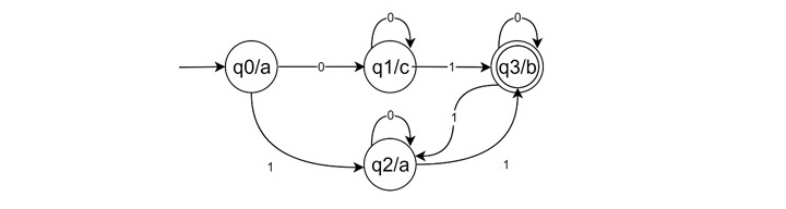
From the above machine, we can determine output from a given input. We can analyse like below −
The machine consists of three states: starting from q0, output are c and a when we are reaching q1 with input 0 and q2 with input 1 respectively.
Similarly from q1, getting input 0 it is in the same state and producing c again; and for 1, moving towards q3 with input b. Like these the q2 and q3 are working.
For input "001101", it will produce −
- Start at q0.
- Input 0: Transition to q1, output c.
- Input 0: stay in q1, output c.
- Input 1: Transition to q3, output b.
- Input 1: Transition to q2, output a.
- Input 0: Stay in q2, output a.
- Input 1: Transition to q3, output b.
So, the output string is "ccbaab"
Example 2
Let us see another example for complementing binary input string through Melay machine.
| Current State | Input | Next State | Output |
|---|---|---|---|
| q0 | 0 | q1 | 1 |
| q0 | 1 | q2 | 0 |
| q1 | 0 | q1 | 1 |
| q1 | 1 | q2 | 0 |
| q2 | 0 | q1 | 1 |
| q2 | 1 | q2 | 0 |
The graph will look like this −
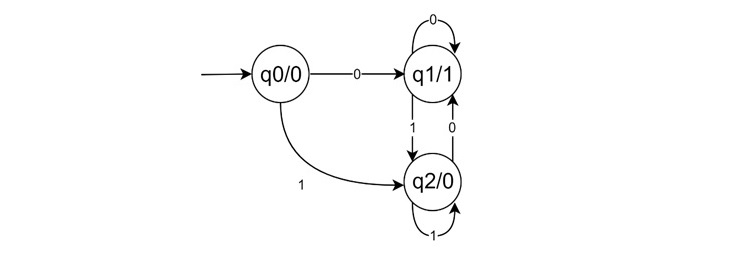
There are three states. For input 0, q1 is responsible and for input 1, q2 is responsible, when it is reaching q1, producing 1 as output and for q2, it is producing 0. So for the input string "011," the output should be "100," which is the 1's complement of the given string.
Conclusion
For finite automata with outputs, we consider the Moore machines. In Moore machines, the outputs are coming with the states, so after reaching a state, we are getting outputs. It is characterized by having an initial state, but no final state.
In this chapter, this article we have seen the structure of Moore machine, how they are formed and then have seen two different examples for Moore machine formation.
