Representation of Turing Machine in Automata Theory

---

---

The Turing Machine is the basic fundamental model of a modern computer. It is an abstract model of computation. It was proposed by Alan Turing in 1936. At that time, there were no computers. The Turing machine can carry out any computational process that a modern computer can perform. It is the machine format of unrestricted language.

In this chapter, we will cover the basic concepts of Turing machine with its representation and examples of how it works.

Basics of Turing Machine

A Turing machine (TM) is defined by 7 tuples: (Q, Σ, Γ, δ, q0, B, F)

• Q − Finite set of states
• Σ − Finite set of input alphabets
• Γ − Finite set of allowable tape symbols
• δ − Transitional function
• q0 − Initial state
• B − A symbol of Γ called blank
• F − Final state

The transitional function δ is a mapping from Q × Γ → (Q Γ × {L, R, H}). This means that from one state, by getting one input from the input tape, the machine moves to a state. It writes a symbol on the tape and moves to left, right, or halts.

Mechanical Diagram of Turing Machine

A Turing machine consists of three main parts: an input tape, a read-write head, finite control.

The input tape contains the input alphabets. It has an infinite number of blanks at the left and right side of the input symbols. The read-write head reads an input symbol from the input tape and sends it to the finite control. The machine must be in some state. In the finite control, the transitional functions are written. Based on the present state and the present input, a suitable transitional function is executed.

Operations of Turing Machine

When a transitional function is executed, the Turing machine performs these operations −

• The machine goes into some state.
• The machine writes a symbol in the cell of the input tape from where the input symbol was scanned.
• The machine moves the reading head to the left or right or halts.

Instantaneous Description (ID) of Turing Machine

The Instantaneous Description (ID) of a Turing machine remembers the following at a given instance of time −

• The contents of all the cells of the tape, starting from the rightmost cell up to at least the last cell, containing a non-blank symbol and containing all cells up to the cell being scanned.
• The cell currently being scanned by the read-write head.
• The state of the machine.

Example of Turing Machine

Let us look at an example of a Turing machine that accepts the language $\mathrm{L \:=\: \{ a^n b^n\:, \:n \:\geq\: 1 \}}$. This language consists of strings with equal number of a's followed by b's, where the number of a's and b's is at least 1.

Transition Functions (B denotes blank)

$$\mathrm{\delta(q0, \: a) \: \rightarrow \: (q1, \: X, \: R)}$$

$$\mathrm{\delta(q1, \: a) \: \rightarrow \: (q1, \: a, \: R)}$$

$$\mathrm{\delta(q1, \: b) \: \rightarrow \: (q2, \: Y, \: L)}$$

$$\mathrm{\delta(q2, \: a) \: \rightarrow \: (q2, \: a, \: L)}$$

$$\mathrm{\delta(q2, \: X) \: \rightarrow \: (q0, \: X, \: R)}$$

$$\mathrm{\delta(q1, \: Y) \: \rightarrow \: (q1, \: Y, \: R)}$$

$$\mathrm{\delta(q2, \: Y) \: \rightarrow \: (q2, \: Y, \: L)}$$

$$\mathrm{\delta(q0, \: Y) \: \rightarrow \: (q3, \: Y, \: R)}$$

$$\mathrm{\delta(q3, \: Y) \: \rightarrow \: (q3, \: Y, \: R)}$$

$$\mathrm{\delta(q3, \: B) \: \rightarrow \: (q4, \: B, \: H)}$$

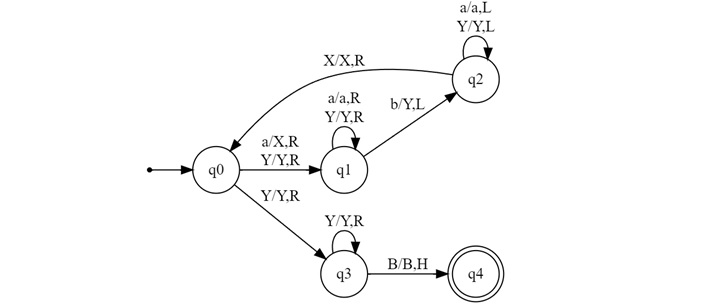
Explanation of Transition Functions

Let's break down how this Turing machine works −

• It starts in state q0 and replaces the first 'a' with 'X'.
• It moves right, keeping 'a's unchanged, until it finds the first 'b'.
• It replaces the first 'b' with 'Y' and moves left.
• It moves left until it finds 'X', then goes back to step 1.
• If it finds 'Y' instead of 'b', it moves right until it finds a blank, then halts in an accepting state.

Instantaneous Description (ID) for the string "aaabbb"

$$\mathrm{BaaabbbB \: \rightarrow \: BXaabbbB}$$

$$\mathrm{BXaabbbB \: \rightarrow \: BXaaYbbB}$$

$$\mathrm{BXaaYbbB \: \rightarrow \: BXXaYbbB}$$

$$\mathrm{BXXaYbbB \: \rightarrow \: BXXaYYbB}$$

$$\mathrm{BXXaYYbB \: \rightarrow \: BXXXYYbB}$$

$$\mathrm{BXXXYYbB \: \rightarrow \: BXXXYYYB \:\:\text{ (Halt in accepting state)}}$$

This ID shows how the Turing machine processes the string "aaabbb" step by step, replacing a's with X's and b's with Y's until it accepts the string.

Conclusion

The Turing machine is a powerful model of computation. It can represent complex languages and perform sophisticated computations. In this chapter, we presented the basic idea of Turing machines with how it works. In addition, we provided suitable state diagram for a machine where it checks equal number of as and bs.