K-dimensional Turing Machine in Automata Theory

---

---

We have seen several variations in Turing machines including multi-tape, multi-head, nondeterministic Turing machines, etc. In this chapter, we will see another variation called Kdimensional Turing machine which is quite interesting in nature. It expands the tape in more than one direction to give more control. Read this chapter to get a clear understanding of how it works.

Basics of K-Dimensional Turing Machine

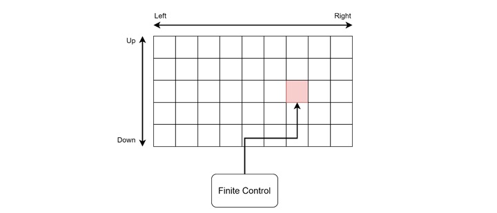
A K-dimensional Turing Machine is a generalization of the standard Turing machine where the tape extends into multiple dimensions. For simplicity, we will discuss a two-dimensional Turing machine (the most common example), the tape can be thought of as a grid that expands infinitely in both the X and Y directions. However, the concept can be extended to any number of dimensions, denoted by K.

The functional block diagram of the machine is looking like below −

Key Characteristics of K-Dimensional Turing Machine

Let us see some of the important characteristics of the K-dimensional Turing machines −

• Multi-dimensional Tape − Unlike the standard one-dimensional tape, the K-dimensional Turing machine has a tape that can extend in K different directions. For example, in a two-dimensional Turing machine, the tape extends both horizontally and vertically.
• Movement Directions − The read-write head can move in any of the available directions within the dimensional space. In a two-dimensional machine, this means the head can move left, right, up, or down.
• Transition Function − The transition function is modified to account for the additional dimensions, directing the machine's movements within the multi-dimensional space.

Why Use K-Dimensional Tapes?

With the complexity of K-dimensional Turing machines we use them because, the primary advantage of a K-dimensional Turing machine is its ability to handle computations that naturally fit into a grid or multi-dimensional structure. This is particularly useful in tasks such as image processing, simulations, and other applications where data is inherently multi-dimensional.

How Does a K-dimensional Turing Machine Work?

A K-dimensional Turing machine operates similarly to a standard Turing machine but with the added complexity of multiple dimensions. The read-write head interacts with the multi-dimensional tape based on a transition function that considers both the current state and the symbols in the relevant cells of the tape.

Transition Function − The transition function for a two-dimensional Turing machine (as an example) can be expressed as −

$$\mathrm{\delta(Q,\: \Sigma)\: \rightarrow\: (Q',\: \Gamma,\: D)}$$

Where −

• Q is the current state of the machine.
• Σ is the symbol read by the head from the current cell.
• Q' is the next state.
• Γ is the symbol to be written in the current cell.
• D indicates the direction in which the head should move (Left, Right, Up, Down).

Example of Navigating a Grid

Let us now take an example where we can use the K-Dimensional (here 2 Dimensional) Turing machine.

Consider a two-dimensional Turing machine that is designed to navigate a grid. The grid contains obstacles that the machine must avoid while moving from a starting point to a destination. The tape extends infinitely in both the X and Y directions, allowing the machine to move freely within the grid.

Initial Configuration

• The grid is mapped onto the two-dimensional tape, with each cell on the grid corresponding to a cell on the tape.
• The machine starts at the initial position, with the head reading the symbol at that location.

Navigating the Grid

• The machine reads the symbol under the head and consults the transition function to determine the next move.
• The head moves in one of four directions (Left, Right, Up, Down) depending on the instructions in the transition function.
• If the head encounters an obstacle (represented by a specific symbol on the tape), the machine changes state and alters its path to avoid the obstacle.

Reaching the Destination

The machine continues to navigate the grid until it reaches the designated destination symbol. At this point, the machine enters a final accepting state, indicating that the task is complete.

Example of Edge Detection

Let us see another example of edge detection, the goal is to identify the boundaries within an image where the intensity of pixels changes sharply.

A two-dimensional Turing machine can be programmed to traverse the grid of pixels, comparing the intensity values of neighboring cells to detect these edges.

• Initialization − The image is loaded onto the two-dimensional tape, with each cell on the tape representing a pixel's intensity value. The machine starts at the top-left corner of the image.
• Edge Detection Algorithm − As the machine moves across the tape, it reads the intensity values of the current pixel and its neighbors.
  • The transition function determines whether the difference in intensity is significant enough to indicate an edge.
  • If an edge is detected, the machine marks the current pixel (or cell) accordingly.
• Output − The machine continues this process for the entire image, eventually producing an output where the edges are highlighted.

Equivalence to Standard Turing Machines

K-dimensional Turing machines have greater flexibility and efficiency for certain tasks. We can convert a K-dimensional machine to a single-dimensional machine as well, since they are computationally equivalent to the standard Turing machine. But still, this is a complex process. Let us see some key points for the conversion.

• Encoding the Multi-dimensional Tape − The K-dimensional tape is encoded onto a one-dimensional tape. This involves mapping each cell in the multi-dimensional space to a unique position on the one-dimensional tape.
• Simulating Movement − The movements of the read-write head in the K-dimensional space are simulated by corresponding movements on the one-dimensional tape.
• Efficiency Considerations − While the conversion is possible, the standard Turing machine may require significantly more steps to perform the same task due to the increased complexity of managing multi-dimensional data on a one-dimensional tape.

Conclusion

In this chapter, we explained the concept of K-Dimensional Turing machine which is more efficient and powerful than the single-head machines. Here we presented two examples to demonstrate how it works.