- Automata Theory - Applications
- Automata Terminology
- Basics of String in Automata
- Set Theory for Automata
- Finite Sets and Infinite Sets
- Algebraic Operations on Sets
- Relations Sets in Automata Theory
- Graph and Tree in Automata Theory
- Transition Table in Automata
- What is Queue Automata?
- Compound Finite Automata
- Complementation Process in DFA
- Closure Properties in Automata
- Concatenation Process in DFA
- Language and Grammars
- Language and Grammar
- Grammars in Theory of Computation
- Language Generated by a Grammar
- Chomsky Classification of Grammars
- Context-Sensitive Languages
- Finite Automata
- What is Finite Automata?
- Finite Automata Types
- Applications of Finite Automata
- Limitations of Finite Automata
- Two-way Deterministic Finite Automata
- Deterministic Finite Automaton (DFA)
- Non-deterministic Finite Automaton (NFA)
- NDFA to DFA Conversion
- Equivalence of NFA and DFA
- Dead State in Finite Automata
- Minimization of DFA
- Automata Moore Machine
- Automata Mealy Machine
- Moore vs Mealy Machines
- Moore to Mealy Machine
- Mealy to Moore Machine
- Myhill–Nerode Theorem
- Mealy Machine for 1’s Complement
- Finite Automata Exercises
- Complement of DFA
- Regular Expressions
- Regular Expression in Automata
- Regular Expression Identities
- Applications of Regular Expression
- Regular Expressions vs Regular Grammar
- Kleene Closure in Automata
- Arden’s Theorem in Automata
- Convert Regular Expression to Finite Automata
- Conversion of Regular Expression to DFA
- Equivalence of Two Finite Automata
- Equivalence of Two Regular Expressions
- Convert Regular Expression to Regular Grammar
- Convert Regular Grammar to Finite Automata
- Pumping Lemma in Theory of Computation
- Pumping Lemma for Regular Grammar
- Pumping Lemma for Regular Expression
- Pumping Lemma for Regular Languages
- Applications of Pumping Lemma
- Closure Properties of Regular Set
- Closure Properties of Regular Language
- Decision Problems for Regular Languages
- Decision Problems for Automata and Grammars
- Conversion of Epsilon-NFA to DFA
- Regular Sets in Theory of Computation
- Context-Free Grammars
- Context-Free Grammars (CFG)
- Derivation Tree
- Parse Tree
- Ambiguity in Context-Free Grammar
- CFG vs Regular Grammar
- Applications of Context-Free Grammar
- Left Recursion and Left Factoring
- Closure Properties of Context Free Languages
- Simplifying Context Free Grammars
- Removal of Useless Symbols in CFG
- Removal Unit Production in CFG
- Removal of Null Productions in CFG
- Linear Grammar
- Chomsky Normal Form (CNF)
- Greibach Normal Form (GNF)
- Pumping Lemma for Context-Free Grammars
- Decision Problems of CFG
- Pushdown Automata
- Pushdown Automata (PDA)
- Pushdown Automata Acceptance
- Deterministic Pushdown Automata
- Non-deterministic Pushdown Automata
- Construction of PDA from CFG
- CFG Equivalent to PDA Conversion
- Pushdown Automata Graphical Notation
- Pushdown Automata and Parsing
- Two-stack Pushdown Automata
- Turing Machines
- Basics of Turing Machine (TM)
- Representation of Turing Machine
- Examples of Turing Machine
- Turing Machine Accepted Languages
- Variations of Turing Machine
- Multi-tape Turing Machine
- Multi-head Turing Machine
- Multitrack Turing Machine
- Non-Deterministic Turing Machine
- Semi-Infinite Tape Turing Machine
- K-dimensional Turing Machine
- Enumerator Turing Machine
- Universal Turing Machine
- Restricted Turing Machine
- Convert Regular Expression to Turing Machine
- Two-stack PDA and Turing Machine
- Turing Machine as Integer Function
- Post–Turing Machine
- Turing Machine for Addition
- Turing Machine for Copying Data
- Turing Machine as Comparator
- Turing Machine for Multiplication
- Turing Machine for Subtraction
- Modifications to Standard Turing Machine
- Linear-Bounded Automata (LBA)
- Church's Thesis for Turing Machine
- Recursively Enumerable Language
- Computability & Undecidability
- Turing Language Decidability
- Undecidable Languages
- Turing Machine and Grammar
- Kuroda Normal Form
- Converting Grammar to Kuroda Normal Form
- Decidability
- Undecidability
- Reducibility
- Halting Problem
- Turing Machine Halting Problem
- Rice's Theorem in Theory of Computation
- Post’s Correspondence Problem (PCP)
- Types of Functions
- Recursive Functions
- Injective Functions
- Surjective Function
- Bijective Function
- Partial Recursive Function
- Total Recursive Function
- Primitive Recursive Function
- μ Recursive Function
- Ackermann’s Function
- Russell’s Paradox
- Gödel Numbering
- Recursive Enumerations
- Kleene's Theorem
- Kleene's Recursion Theorem
- Advanced Concepts
- Matrix Grammars
- Probabilistic Finite Automata
- Cellular Automata
- Reduction of CFG
- Reduction Theorem
- Regular expression to ∈-NFA
- Quotient Operation
- Parikh’s Theorem
- Ladner’s Theorem
Moore to Mealy Machine Conversion
Both Mealy and Moore machines generate outputs from the finite state machine. In this chapter, we will explain how to convert a Moore machine to a Mealy machine. We'll use the state diagram of the Moore machine as our starting point and learn how to convert it into the equivalent state diagram of the Mealy machine.
Concepts for Moore and Mealy Machines
In a Moore machine, the output is represented on the state itself. In contrast, in a Mealy machine, the output is represented on the transition, or in other words, on the arrow itself.
Compared to the Mealy-to-Moore conversion, this Moore-to-Mealy conversion is relatively simple. Let us take a look at the conversion rules.
Basic Conversion Rules
Converting a Moore machine to a Mealy machine is simple. The key is to transfer the output information from the states in the Moore diagram to the transition arrows in the Mealy diagram. Here are the rules −
Rule 1: Incoming Transitions
For each state in the Moore diagram, check its incoming transitions.
Imagine a state 'A' with two incoming transitions. In one transition, the input is '0', while in the second transition, the input is '1'. Let's say the output of the machine in state 'A' is '1'.

In the equivalent Mealy representation, we'll write the '1' alongside the input for both transitions. This '1' represents the output during each transition leading to state 'A'.

If the output of the machine in state 'A' was '0' instead of '1', we would write '0' alongside the input for both transitions.
Rule 2: Outgoing Transitions and Outputs
Once we've covered all the incoming transitions to a state, we move on to the outgoing transitions from that specific state.
Let's say state 'A' has two outgoing transitions. Imagine the output '1' is within state 'A' itself, and there's a transition from 'A' to state 'B'.

In the equivalent Mealy diagram, the transition looping back to state 'A' will have the output '1' associated with it, as that's the output of the machine in state 'A'.

The outgoing transition from 'A' to 'B' will have the output associated with state 'B' in the Moore diagram. If state 'B' has an output of '0', then the transition from 'A' to 'B' will have '0' written on it in the Mealy diagram.
Example of Moore to Mealy Machine Conversion
Let us understand the idea through an example for a better understanding. Consider we have a Moore machine state diagram with three states.

State Transition Table
The state transition table is like below −
| State | Output | Input = 0 | Input = 1 |
|---|---|---|---|
| A | 1 | C | A |
| B | 0 | C | A |
| C | 0 | A | B |
Now let us try to make the Mealy machine diagram corresponding to the previous Moore diagram.
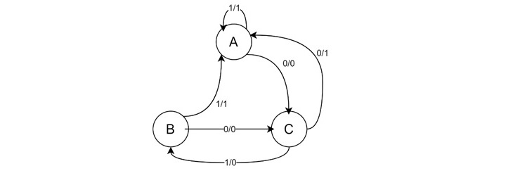
| PS | Next State (X = 0) | Next State (X = 1) | Output (X = 0) | Output (X = 1) |
|---|---|---|---|---|
| A | C | A | 0 | 1 |
| B | C | A | 0 | 1 |
| C | A | B | 1 | 0 |
When we convert a Moore machine to a Mealy machine, the number of states in the equivalent Mealy machine will be less than or equal to the Moore machine.
After converting the Moore machine to a Mealy machine, it's essential to check for redundant states in the state diagram.
- Identify Identical Rows − Analyze the state table for rows with identical next states and outputs for each input. These rows indicate redundant states.
- Remove Redundant States − Choose one of the redundant states and replace all its instances in the state table and diagram with the other identical state.
- Simplified State Diagram − The resulting state diagram with the removed redundant state represents the simplified Mealy machine.

Let us see another example with five states.
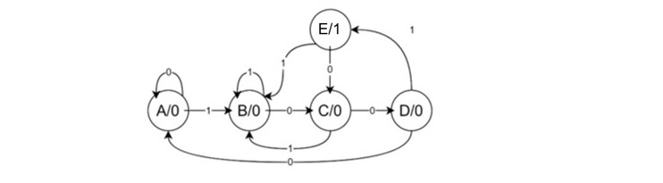
| State | Output | Input = 0 | Input = 1 |
|---|---|---|---|
| A | 0 | A | B |
| B | 0 | C | B |
| C | 0 | D | B |
| D | 0 | A | E |
| E | 1 | C | B |
Now let us convert to Mealy −
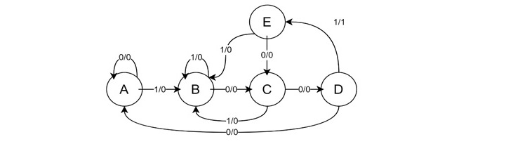
| PS | Next State (X=0) | Next State (X=1) | Output (X=0) | Output (X=1) |
|---|---|---|---|---|
| A | A | B | 0 | 0 |
| B | C | B | 0 | 0 |
| C | D | B | 0 | 0 |
| D | A | E | 0 | 1 |
| E | C | B | 0 | 0 |
In the table, the states 'B' and 'E' have identical next states and outputs for both input values (0 and 1). So we can reduce them by removing state 'E' from the state table and diagram, replacing its instances with state 'B'.

| PS | Next State (X=0) | Next State (X=1) | Output (X=0) | Output (X=1) |
|---|---|---|---|---|
| A | A | B | 0 | 0 |
| B | C | B | 0 | 0 |
| C | D | B | 0 | 0 |
| D | A | B | 0 | 1 |
Conclusion
Converting a Moore machine to a Mealy machine is a straightforward process. We just need to analyze the incoming and outgoing transitions carefully and then associate the output based on the states in the original Moore diagram.
After the conversion, we should check for and remove redundant states to obtain a simplified and efficient Mealy machine representation to make it efficient.
