Turing Machine for Addition in Automata Theory

Quiz

In this chapter, we will present the concept of using a Turing Machine to perform addition operation of two integers. The Turing Machine is a powerful theoretical model used in computer science to understand computation.

Turing Machine can be used for simple tasks like addition. Here, we will break down the steps involved in using a Turing Machine for adding two integers, and we will also take an example to demonstrate how it is done.

Introduction to Turing Machines

In the basic Turing Machine, there is an infinite tape divided into cells, each containing a symbol from a finite alphabet. The machine has a head that reads and writes symbols on the tape and can move left or right, depending on the rules defined by a transition function.

Turing Machines can be thought of as a basic computer that, given an input on its tape, follows a set of rules to manipulate that input until it reaches a final state.

Basic Structure of a Turing Machine for Addition

To perform addition using a Turing Machine, we need to encode the numbers on the tape in a way that the machine can process. Typically, we use a series of symbols, such as '0' to represent the numbers, and a separator, like 'B' (for blank), to separate the numbers.

For example, if we want to add two numbers, x and y, we represent them on the tape as −

$$\mathrm{0^x \:B0^y}$$

Here, 0^x represents the first number with x number of 0s, B is the separator, and 0^y represents the second number with y number of 0s.

Step-by-Step Addition Process

Let us see how the addition can be performed. We need to follow these steps.

Traverse the First Number − The machine begins by traversing the first number (0^x) until it reaches the separator B.
Replace the Separator − Upon reaching B, the machine changes the state and replaces B with 0, effectively merging the two series of zeros.
Traverse the Second Number − The machine then moves through the second series of zeros (0^y).
End of Addition − When the machine reaches the end of the second number, it replaces the last 0 with B and halts. The final state of the tape represents the sum of the two numbers.

Let's look at the Turing Machine's transition diagram for this process −

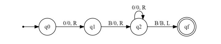
The stat transition diagram may look a little confusing but it will be easier for us if we go through an example

Example: Adding Two Numbers

Let us work through an example using the Turing Machine. We want to add 3 and 2. Here is how we would represent this on the tape and how the Turing Machine would process it.

Initial Tape − The tape begins with 0³B0² = 000B00.

Steps

Initial State (q0) − The machine starts at the beginning of the tape and is in state q0. It reads the first 0 and moves right, staying in state q0.
Traverse First Number − The machine continues moving right, reading each 0 until it encounters B, transitioning to state q1.
Replace Separator − Upon encountering B, the machine changes the state to q1, and it replaces B with 0. The tape now reads 000000.
Traverse Second Number − The machine moves right, reading each 0 until it encounters B. It then transitions to state qf.
Final State − In state qf, the machine halts. The tape now reads 00000, which represents the sum, 5.

Implementing Function with Addition

In addition to adding two separate integers, a Turing Machine can also be designed to perform operations like adding a constant value to a single integer. In this section, we will explore how a Turing Machine can compute the function f(x) = x + 2.

Representation of the Input

To represent the integer x on the Turing Machine's tape, we use a sequence of zeros, similar to how we represented numbers in the previous section.

The input for the function f(x) = x + 2 is written as −

$$\mathrm{O^{x}B}$$

Here, 0x represents the integer xxx, and B is the blank space that follows the number.

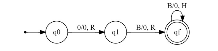
Step-by-Step Process to Compute f(x) = x+2

The Turing Machine calculates f(x) = x + 2 by following these steps −

Traverse the Input Number − The machine begins at the leftmost part of the tape and traverses the sequence of zeros representing x until it encounters the blank B.
Add the First Zero − Upon reaching B, the machine changes its state and replaces B with 0, effectively adding one zero to the end of the sequence.
Add the Second Zero − The machine continues moving right and encounters another B after the first added zero. It again changes the state and replaces this B with another 0, adding the second zero.
Halt − Finally, the machine halts with the tape containing x + 2 zeros.

Let's illustrate this process with the corresponding transition diagram −

Construct Turing Machine for Fddition

Generally in different finite automata a number is represented in binary format.

Example: 2- 010

$$\mathrm{3 - \:011}$$

$$\mathrm{4 - \:100}$$

But in case of addition using the Turing machine the system follows a unary format.

Example: 2- 11 or 00

$$\mathrm{3- \: 111 \:or\: 000}$$

$$\mathrm{4- \:1111 \:or\: 0000}$$

In unary format a number is represented

So, let's consider zero's to represent any number in the Turing machine for doing addition.

Example: Inputs 4 and 5

$$\mathrm{4 \:=\: 0000}$$

$$\mathrm{5 \:=\: 00000}$$

$$\mathrm{\text{Then }\: 4 \:+\: 5 \:=\: 0000c00000}$$

Both numbers are separated by a temporary variable c for representing the two numbers

Output

$$\mathrm{000000000 \:=\: 9}$$

The Turing Machine (TM) is as follows −

Explanation

Step 1 − convert 0 into X jump to step 3.

Step 2 − If the symbol is "c" then convert it into blank, move right and jump to step-6.

Step 3 − Ignore 0's and move towards the right. Ignore "c", and then move right

Step 4 − Ignore 0's and move towards the right. Convert a Blank into 0, and then move left

Step 5 − Ignore 0's and move towards the left.

Step 6 − Ignore "c", move left.

Step 7 − Ignore 0's and move towards left.

Step 8 − Ignore an X, move left and jump to step 1.

Conclusion

Turing machine can solve any problem that can be solvable using polynomial time algorithms. In this chapter, we explained how the Turing Machine can be used for addition and addition-based functions as well. We presented the steps along with the state transition diagrams with example for a clear understanding.

Print Page