- Automata Theory - Applications
- Automata Terminology
- Basics of String in Automata
- Set Theory for Automata
- Finite Sets and Infinite Sets
- Algebraic Operations on Sets
- Relations Sets in Automata Theory
- Graph and Tree in Automata Theory
- Transition Table in Automata
- What is Queue Automata?
- Compound Finite Automata
- Complementation Process in DFA
- Closure Properties in Automata
- Concatenation Process in DFA
- Language and Grammars
- Language and Grammar
- Grammars in Theory of Computation
- Language Generated by a Grammar
- Chomsky Classification of Grammars
- Context-Sensitive Languages
- Finite Automata
- What is Finite Automata?
- Finite Automata Types
- Applications of Finite Automata
- Limitations of Finite Automata
- Two-way Deterministic Finite Automata
- Deterministic Finite Automaton (DFA)
- Non-deterministic Finite Automaton (NFA)
- NDFA to DFA Conversion
- Equivalence of NFA and DFA
- Dead State in Finite Automata
- Minimization of DFA
- Automata Moore Machine
- Automata Mealy Machine
- Moore vs Mealy Machines
- Moore to Mealy Machine
- Mealy to Moore Machine
- Myhill–Nerode Theorem
- Mealy Machine for 1’s Complement
- Finite Automata Exercises
- Complement of DFA
- Regular Expressions
- Regular Expression in Automata
- Regular Expression Identities
- Applications of Regular Expression
- Regular Expressions vs Regular Grammar
- Kleene Closure in Automata
- Arden’s Theorem in Automata
- Convert Regular Expression to Finite Automata
- Conversion of Regular Expression to DFA
- Equivalence of Two Finite Automata
- Equivalence of Two Regular Expressions
- Convert Regular Expression to Regular Grammar
- Convert Regular Grammar to Finite Automata
- Pumping Lemma in Theory of Computation
- Pumping Lemma for Regular Grammar
- Pumping Lemma for Regular Expression
- Pumping Lemma for Regular Languages
- Applications of Pumping Lemma
- Closure Properties of Regular Set
- Closure Properties of Regular Language
- Decision Problems for Regular Languages
- Decision Problems for Automata and Grammars
- Conversion of Epsilon-NFA to DFA
- Regular Sets in Theory of Computation
- Context-Free Grammars
- Context-Free Grammars (CFG)
- Derivation Tree
- Parse Tree
- Ambiguity in Context-Free Grammar
- CFG vs Regular Grammar
- Applications of Context-Free Grammar
- Left Recursion and Left Factoring
- Closure Properties of Context Free Languages
- Simplifying Context Free Grammars
- Removal of Useless Symbols in CFG
- Removal Unit Production in CFG
- Removal of Null Productions in CFG
- Linear Grammar
- Chomsky Normal Form (CNF)
- Greibach Normal Form (GNF)
- Pumping Lemma for Context-Free Grammars
- Decision Problems of CFG
- Pushdown Automata
- Pushdown Automata (PDA)
- Pushdown Automata Acceptance
- Deterministic Pushdown Automata
- Non-deterministic Pushdown Automata
- Construction of PDA from CFG
- CFG Equivalent to PDA Conversion
- Pushdown Automata Graphical Notation
- Pushdown Automata and Parsing
- Two-stack Pushdown Automata
- Turing Machines
- Basics of Turing Machine (TM)
- Representation of Turing Machine
- Examples of Turing Machine
- Turing Machine Accepted Languages
- Variations of Turing Machine
- Multi-tape Turing Machine
- Multi-head Turing Machine
- Multitrack Turing Machine
- Non-Deterministic Turing Machine
- Semi-Infinite Tape Turing Machine
- K-dimensional Turing Machine
- Enumerator Turing Machine
- Universal Turing Machine
- Restricted Turing Machine
- Convert Regular Expression to Turing Machine
- Two-stack PDA and Turing Machine
- Turing Machine as Integer Function
- Post–Turing Machine
- Turing Machine for Addition
- Turing Machine for Copying Data
- Turing Machine as Comparator
- Turing Machine for Multiplication
- Turing Machine for Subtraction
- Modifications to Standard Turing Machine
- Linear-Bounded Automata (LBA)
- Church's Thesis for Turing Machine
- Recursively Enumerable Language
- Computability & Undecidability
- Turing Language Decidability
- Undecidable Languages
- Turing Machine and Grammar
- Kuroda Normal Form
- Converting Grammar to Kuroda Normal Form
- Decidability
- Undecidability
- Reducibility
- Halting Problem
- Turing Machine Halting Problem
- Rice's Theorem in Theory of Computation
- Post’s Correspondence Problem (PCP)
- Types of Functions
- Recursive Functions
- Injective Functions
- Surjective Function
- Bijective Function
- Partial Recursive Function
- Total Recursive Function
- Primitive Recursive Function
- μ Recursive Function
- Ackermann’s Function
- Russell’s Paradox
- Gödel Numbering
- Recursive Enumerations
- Kleene's Theorem
- Kleene's Recursion Theorem
- Advanced Concepts
- Matrix Grammars
- Probabilistic Finite Automata
- Cellular Automata
- Reduction of CFG
- Reduction Theorem
- Regular expression to ∈-NFA
- Quotient Operation
- Parikh’s Theorem
- Ladner’s Theorem
Turing Machine for Multiplication in Automata Theory
In this chapter, we will explain how to design a Turing machine that can perform multiplication of two numbers. The numbers will be unary numbers as we are using in other examples as well. We start with the basics and then get a detailed example with steps for a better understanding of the concept.
Basics of Turing Machine Multiplication
We know the Turing Machines are used to solve problems that can be solved through polynomial time algorithms. In other words, it can simulate the logic of any computer algorithm. In our case, we will use it to multiply two numbers which is also a straightforward operation.
Representing Numbers
In a Turing machine, we use the unary number system. This means −
- The number 2 is represented as "11"
- The number 3 is represented as "111"
Multiplication Logic
The key idea is to use repeated addition. For example −
- 2 × 3 = 3 + 3
- We add 3 to itself 2 times
Detailed Example: Multiplying 2 × 3
Let us walk through the process of designing a Turing machine to multiply 2 and 3.
Initial Tape Setup
Our Turing machine tape will look like this at the start −
$$\mathrm{110111}$$
The first "11" represents 2. The "111" after the separator represents 3. Between these two, the "0" is there for a separator. And the remaining tape is blank. We leave blank space for the result.
Step-by-Step Process
The steps are as follows –
- Cancel the First '1' − We start by canceling the first '1' from the first number (2). This helps us keep track of how many times we need to add.
- Copy the Second Number − We copy the pattern "111" (representing 3) to the result area. We use a special marker (let's call it 'Y') to remember where we copied from.
- Repeat and Add − We go back to the first number. If there is still a '1', we repeat the process. This means we will add 3 again to our result.
- Cleanup − After all, '1's from the first number are used, we clean up. We remove the original numbers and separators. We are left with just the result on the tape.
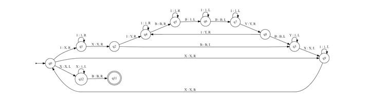
Detailed Turing Machine States
Here is the detailed State Diagram –
Detailed Turing Machine Transition Table
Here is the detailed Transition Table –
| Current State | Input Symbol | Next State | Output | Move |
|---|---|---|---|---|
| q0 | 1 | q1 | X | Right |
| q0 | X | q9 | X | Right |
| q0 | X | q12 | X | Left |
| q1 | 1 | q1 | 1 | Right |
| q1 | X | q2 | X | Right |
| q12 | X | q12 | 1 | Left |
| q12 | B | q11 | B | Right |
| q9 | 1 | q9 | 1 | Left |
| q9 | X | q0 | X | Right |
| q2 | 1 | q4 | Y | Right |
| q3 | Y | q3 | 1 | Left |
| q8 | B | q3 | B | Left |
| q7 | Y | q8 | Y | Right |
| q4 | 1 | q4 | 1 | Right |
| q4 | B | q5 | B | Right |
| q5 | 1 | q5 | 1 | Right |
| q5 | B | q6 | 1 | Left |
| q6 | 1 | q6 | 1 | Left |
| q7 | 1 | q7 | 1 | Left |
| q6 | B | q7 | B | Left |
| q3 | X | q9 | X | Left |
| q2 | B | q3 | B | Left |
| q8 | 1 | q4 | Y | Right |
Explanations
- q0 (Start and Main Loop) − Begins by scanning for the first unprocessed symbol in the input. If it encounters a '1', it knows it's in the first factor and transitions to q1. If it encounters an 'X', it moves right (staying in q0) to continue the search. If it encounters a 'B' (blank), it means the first factor is fully processed, and it transitions to q12.
- q1 (Process '1' in First Factor) − Skips over any '1's in the first factor, moving right until it finds the separating 'X'.
- q2 (Found Separator) − Marks that the current digit of the first factor is processed. Transitions to q3 without changing the tape.
- q3 (Reset Second Factor) − Converts any 'Y's (marking processed '1's in the second factor) back to '1's. Prepares for the next iteration by moving left until it encounters an 'X' (marking processed '1's in the first factor).
- q4 (Process '1' in Second Factor) − Found a '1' in the second factor. Replaces the '1' with a 'Y' to mark it as processed. Moves right to add a '1' to the result at the end of the tape.
- q5 (Add to Result) − Skips over any existing '1's in the result, moving right. When it encounters a 'B' (blank), it writes a '1' to represent adding one to the product. Then, it transitions to q6 to move back left.
- q6, q7 (Return to Second Factor) − These states guide the machine leftward, skipping over '1's representing the product and the second factor until reaching the beginning of the second factor again.
- q8 (Found Processed '1' in Second Factor) − Encounters a 'Y', indicating a '1' in the second factor was used. Transitions to q4 to process this '1' again (for the next digit of the first factor).
- q9 (Return to Next Digit in First Factor) − Skips over any '1's in the first factor, moving right, to find the next unprocessed '1'. Transitions back to q0 to continue the main loop.
- q12 (First Factor Consumed) − Converts all the 'X's back to '1's to reset the first factor for potential future multiplications. Transitions to q11, signalling that the multiplication is complete.
- q11 (Halt) − Represents the halting state. The tape now contains the product of the input numbers.
Conclusion
Multiplication is a complex process with around 12 to 13 different states. In this chapter, we demonstrated step-by-step how you can use a Turing machine to multiple two numbers. We also presented the state diagram and the transition table for an easy understanding.
