Reduction Theorem in TOC

---

---

The Reduction Theorem is an important idea used in complexity classes theorems. It helps to understand how problems relate to each other in terms of their complexity. In this chapter, we will understand the basics of the Reduction Theorem, and its importance, and see at several examples for a better understanding of their applications.

Reduction Theorem

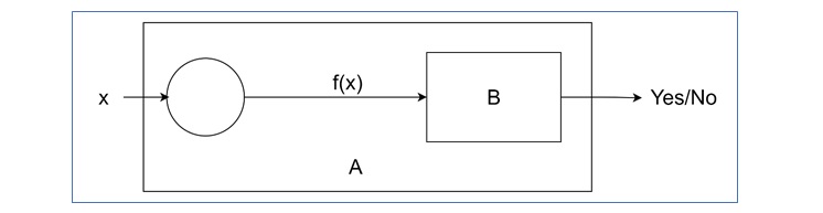
To define the reduction, we can explain this formally like, the reduction theorem involves a function that maps one problem to another.

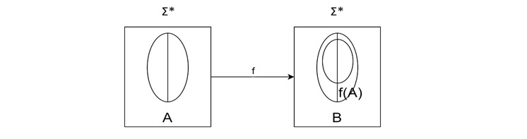
Formally, a reduction from A to B is a function f : Σ₁* → Σ₂* such that for any w ∈ Σ₁* , w ∈ A if and only if f(w) ∈ B.

In simpler terms −

• Every w ∈ A maps to some f(w) ∈ B.
• Every w ∉ A maps to some f(w) ∉ B.
• The function f does not have to be injective or surjective.

We use the following notations to represent reductions −

• A <= B: Problem A is reducible to problem B.
• A <=m B: Problem A is many-to-one reducible to problem B.
• A <=p B: Problem A is reducible in a polynomial manner to problem B.

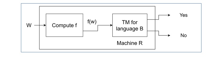
Reductions are important because they allow us to relate the difficulty of different problems. If language A reduces to language B, we can use a recognizer, co-recognizer, or decider for B to recognize, co-recognize, or decide problem A.

When we say A is reducible to B (A <= B), it indicates that problem B is at least as hard as problem A. This helps us categorize problems based on their complexity.

Mapping Reductions

A mapping reduction is a specific type of reduction. It's defined as follows −

A function f : Σ₁* → Σ₂* is called a mapping reduction from A to B if −

• For any w ∈ Σ₁* , w ∈ A if and only if f(w) ∈ B.
• f is a computable function.

A mapping reduction from A to B means that a computer can transform any instance of A into an instance of B such that the answer to B is the answer to A.

Properties of Reduction

Let us see the properties of reduction. Some key properties are listed below −

• If A <= B and A is undecidable, then B is also undecidable.
• If A <= B and B is decidable, then A is also decidable.
• If A <= B and B is recursive, then A is also recursive.
• If A <= B and B is recursively enumerable, then A is also recursively enumerable.
• If A <= B and B is a P-problem, then A is also a P-problem.
• If A <= B and B is an NP-problem, then A is also an NP-problem.
• If A <= B and B <= C, then A <= C (transitivity).
• If A <= B and B <= A, then A and B are polynomially equivalent.
• If A <= B and A is not recursively enumerable, then B is also not recursively enumerable.
• If A <= B and A is not a P-problem, then B is also not a P-problem.
• If A <= B and A is not a recursive problem, then B is also not a recursive problem.

Examples of Reduction Theorem

Let us see some examples to understand how reduction works.

Example 1: Mathematical Reduction

Consider the following reduction −

$$\mathrm{A \: :\: t^4 \:-\: 1 \quad \text{reduces to} \quad B \: : \:t^2 \:-\: 1 \quad \text{and} \quad C \: : \: t^2 \: +\: 1}$$

Here, A is solvable, and since B and C < A, both B and C are also solvable. We can see this because −

$$\mathrm{(t^4 \:-\: 1) \:=\: (t^2 \:-\: 1)(t^2 \:+\: 1)}$$

Example 2: Language Problem Reduction

Problem A: Is L(D) = Σ* ? This can be reduced to: Problem B: Is L(D₁) = Σ* - L(D₂)?

In this case, B is a subset of A, so A is reduced to Problem B.

Example 3: Grammar Problem Reduction

Problem A: Is L(G) = NULL? This can be reduced to: Problem B: Is L(G₁) a subset of L(G₂)?

By reducing Problem A to the simpler Problem B, we can find an easier solution.

Example 4: Polynomial Reduction

$\mathrm{A \: :\: a^3 \:+\: b^3 \:+\: 3a^2b \:+\: 3b^2a \quad \text{can be reduced to} \quad B\: :\: (a \:+\: b)^3}$

If A reduces to B and B is "solvable," then A is also "solvable."

Example 5: Language Reduction

Reduction of L to 01: W = 01 and W = 10

The reduced form f(w) will be −

$$\mathrm{f(w) \:=\: \begin{cases} 01 & \text{if } w \in L, \\ 10 & \text{if } w \notin L \end{cases}}$$

Example 6: Grammar Reduction

Given a grammar G with production rules −

$\mathrm{P \: : \:S\: \rightarrow \:AC\: \mid \:B, \quad A\: \rightarrow \:a, \quad C\: \rightarrow\: c\: \mid\: BC, \quad E\: \rightarrow\: aA\: \mid\: e}$

We can reduce it to an equivalent grammar G' in two phases −

$\mathrm{\text{Phase 1: } \:G' \:=\: \{(A,\: C,\: E,\: S),\: (A,\: C,\: E),\: P,\: (S) \}, \quad P \: :\: S \: \rightarrow \: AC, \quad A\: \rightarrow\: a, \quad C \:\rightarrow\: c, \quad E\: \rightarrow\: aA\: \mid\: e}$

$\mathrm{\text{Phase 2: }\: G''\: =\: \{ (A,\: C,\: S),\: (a,\: c),\: P,\: \{ S \} \}, \quad P\: :\: S\: \rightarrow \: AC, \quad A\: \rightarrow \:a, \quad C\: \rightarrow\: c}$

Example 7: Real-World Problem Reduction

Problem A (Hard Problem): Move from New Guinea to Amazon City. We know there's an easy way from New Guinea to Canada, so we can reduce this to: Problem B (Easier Problem): Move from Canada to Amazon City.

This example shows how we can reduce a hard problem to an easier one. If we can solve the easier problem, we can use that solution to solve the harder one.

Example 8: Decidability Reduction

Given Problem,

$$\mathrm{A \: :\: L_1\: \leq \:L_3\: \text{ and }\: L_2\: \leq\: L_3}$$

We can deduce −

If L₃ is decidable, then L₁ is decidable and L₂ is either decidable or not decidable.

If L₃ is unde cidable, then L₁ is either decidable or not decidable and L₃ is undecidable.

Conclusion

In this chapter, we explained the concept of Reduction Theorem in Automata. We discussed the meaning of reduction and why it matters in computational theory. We then looked at mapping reductions and the important properties of reductions. We covered several examples from simple mathematical reductions to more complex language and grammar problems.