- Automata Theory - Applications
- Automata Terminology
- Basics of String in Automata
- Set Theory for Automata
- Finite Sets and Infinite Sets
- Algebraic Operations on Sets
- Relations Sets in Automata Theory
- Graph and Tree in Automata Theory
- Transition Table in Automata
- What is Queue Automata?
- Compound Finite Automata
- Complementation Process in DFA
- Closure Properties in Automata
- Concatenation Process in DFA
- Language and Grammars
- Language and Grammar
- Grammars in Theory of Computation
- Language Generated by a Grammar
- Chomsky Classification of Grammars
- Context-Sensitive Languages
- Finite Automata
- What is Finite Automata?
- Finite Automata Types
- Applications of Finite Automata
- Limitations of Finite Automata
- Two-way Deterministic Finite Automata
- Deterministic Finite Automaton (DFA)
- Non-deterministic Finite Automaton (NFA)
- NDFA to DFA Conversion
- Equivalence of NFA and DFA
- Dead State in Finite Automata
- Minimization of DFA
- Automata Moore Machine
- Automata Mealy Machine
- Moore vs Mealy Machines
- Moore to Mealy Machine
- Mealy to Moore Machine
- Myhill–Nerode Theorem
- Mealy Machine for 1’s Complement
- Finite Automata Exercises
- Complement of DFA
- Regular Expressions
- Regular Expression in Automata
- Regular Expression Identities
- Applications of Regular Expression
- Regular Expressions vs Regular Grammar
- Kleene Closure in Automata
- Arden’s Theorem in Automata
- Convert Regular Expression to Finite Automata
- Conversion of Regular Expression to DFA
- Equivalence of Two Finite Automata
- Equivalence of Two Regular Expressions
- Convert Regular Expression to Regular Grammar
- Convert Regular Grammar to Finite Automata
- Pumping Lemma in Theory of Computation
- Pumping Lemma for Regular Grammar
- Pumping Lemma for Regular Expression
- Pumping Lemma for Regular Languages
- Applications of Pumping Lemma
- Closure Properties of Regular Set
- Closure Properties of Regular Language
- Decision Problems for Regular Languages
- Decision Problems for Automata and Grammars
- Conversion of Epsilon-NFA to DFA
- Regular Sets in Theory of Computation
- Context-Free Grammars
- Context-Free Grammars (CFG)
- Derivation Tree
- Parse Tree
- Ambiguity in Context-Free Grammar
- CFG vs Regular Grammar
- Applications of Context-Free Grammar
- Left Recursion and Left Factoring
- Closure Properties of Context Free Languages
- Simplifying Context Free Grammars
- Removal of Useless Symbols in CFG
- Removal Unit Production in CFG
- Removal of Null Productions in CFG
- Linear Grammar
- Chomsky Normal Form (CNF)
- Greibach Normal Form (GNF)
- Pumping Lemma for Context-Free Grammars
- Decision Problems of CFG
- Pushdown Automata
- Pushdown Automata (PDA)
- Pushdown Automata Acceptance
- Deterministic Pushdown Automata
- Non-deterministic Pushdown Automata
- Construction of PDA from CFG
- CFG Equivalent to PDA Conversion
- Pushdown Automata Graphical Notation
- Pushdown Automata and Parsing
- Two-stack Pushdown Automata
- Turing Machines
- Basics of Turing Machine (TM)
- Representation of Turing Machine
- Examples of Turing Machine
- Turing Machine Accepted Languages
- Variations of Turing Machine
- Multi-tape Turing Machine
- Multi-head Turing Machine
- Multitrack Turing Machine
- Non-Deterministic Turing Machine
- Semi-Infinite Tape Turing Machine
- K-dimensional Turing Machine
- Enumerator Turing Machine
- Universal Turing Machine
- Restricted Turing Machine
- Convert Regular Expression to Turing Machine
- Two-stack PDA and Turing Machine
- Turing Machine as Integer Function
- Post–Turing Machine
- Turing Machine for Addition
- Turing Machine for Copying Data
- Turing Machine as Comparator
- Turing Machine for Multiplication
- Turing Machine for Subtraction
- Modifications to Standard Turing Machine
- Linear-Bounded Automata (LBA)
- Church's Thesis for Turing Machine
- Recursively Enumerable Language
- Computability & Undecidability
- Turing Language Decidability
- Undecidable Languages
- Turing Machine and Grammar
- Kuroda Normal Form
- Converting Grammar to Kuroda Normal Form
- Decidability
- Undecidability
- Reducibility
- Halting Problem
- Turing Machine Halting Problem
- Rice's Theorem in Theory of Computation
- Post’s Correspondence Problem (PCP)
- Types of Functions
- Recursive Functions
- Injective Functions
- Surjective Function
- Bijective Function
- Partial Recursive Function
- Total Recursive Function
- Primitive Recursive Function
- μ Recursive Function
- Ackermann’s Function
- Russell’s Paradox
- Gödel Numbering
- Recursive Enumerations
- Kleene's Theorem
- Kleene's Recursion Theorem
- Advanced Concepts
- Matrix Grammars
- Probabilistic Finite Automata
- Cellular Automata
- Reduction of CFG
- Reduction Theorem
- Regular expression to ∈-NFA
- Quotient Operation
- Parikh’s Theorem
- Ladner’s Theorem
Turing Machine as Comparator in Automata Theory
Read this chapter to learn how a Turing Machine can be used as a comparator. We will see how the input can be put inside the tape and check the corresponding inputs for comparison. We will see the steps in detail with examples for a clear understanding.
Turing Machine as a Comparator
A Turing Machine can perform various operations, including comparing two numbers to determine if they are equal, less than, or greater than each other.
This concept is similar to how Turing Machines handle addition and subtraction. Let us see how, we will use unary numbers to as input to a Turing Machine to work as a comparator. The basic logic and structure of the Turing Machine remain consistent with those used in other operations.
Unary Numbers
As we know, unary numbers represent quantities using repeated symbols, typically the digit "1." For instance, the number 3 is represented as "111" in unary, and 2 is represented as "11". We will use a "0" as a separator between the two numbers we want to compare.
Example: Comparing Two Numbers
Setting up the Problem − Let us start by comparing two numbers using a Turing Machine. We will work with the following example −
- Number A: "111" (which represents 3)
- Number B: "111" (which also represents 3)
In this case, we have a "0" separating the two numbers: "1110111".
The Process of Comparison − The Turing Machine begins by scanning the tape from the leftmost "1". Here is a step-by-step breakdown of the process −
- Convert the First "1" in A to "X" − The machine reads the first "1" in the left-hand side number (A) and converts it into an "X". This indicates that this digit has been processed.
- Move to the First "1" in B and Convert It to "X" − After processing the first "1" in A, the machine moves right, skipping any "1"s until it encounters the separator "0". It then continues moving right to find the first "1" in the right-hand side number (B) and converts it into an "X".
- Repeat the Process − The machine moves back to the left to find the next unprocessed "1" in A, converts it into an "X", and repeats the process for the next unprocessed "1" in B. This cycle continues until all "1"s in both numbers have been converted to "X".
Handling Different Outcomes
There are three final states: for equal case, for first one greater than the second, and for the second one greater than the first one.
Case 1: A Equal to B − If both numbers have the same number of "1"s, the machine will convert all "1"s in both A and B into "X". After processing, if the machine encounters only "X"s and no additional "1"s in either number, it concludes that A is equal to B.
Case 2: A Less Than B − If A has fewer "1"s than B, the machine will encounter an extra "1" in B after all "1"s in A have been processed. This extra "1" indicates that A is less than B.
Case 3: A Greater Than B − If A has more "1"s than B, the machine will continue processing "1"s in A even after all "1"s in B have been converted to "X". When the machine encounters a blank space (indicating the end of B) while A still has unprocessed "1"s, it concludes that A is greater than B.
Transition Diagram Construction
Once the logic is understood, constructing the transition diagram for the Turing Machine as a comparator becomes straightforward. The states and transitions follow the process described above, with each state representing a step in the comparison process.
State Transitions Diagram
The state transitions diagram looks like this −
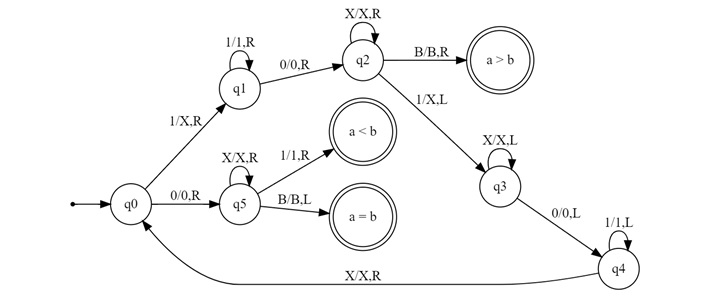
Transition Table
Here is its Transition Table
| Current State | Symbol Read | New State | Write Symbol | Move |
|---|---|---|---|---|
| q0 | 1 | q1 | X | R |
| q0 | X | q4 | X | R |
| q0 | 0 | q5 | 0 | R |
| q1 | 1 | q1 | 1 | R |
| q1 | 0 | q2 | 0 | R |
| q2 | X | q2 | X | R |
| q2 | B | q (a > b) | B | R |
| q2 | 1 | q3 | X | L |
| q3 | X | q3 | X | L |
| q3 | 0 | q4 | 0 | L |
| q4 | 1 | q4 | 1 | L |
| q4 | X | q0 | X | R |
| q5 | X | q5 | X | R |
| q5 | 1 | q (a < b) | 1 | R |
| q5 | B | q (a = b) | B | L |
- Q0 (Initial State) − On reading "1", convert it to "X", and move right. Continue moving right until encountering "0" (separator).
- Q1 − On reading "0", move right. On reading "1" in B, convert it to "X" and move left.
- Q2 − Move left to find the next unprocessed "1" in A. On finding "X" or "0", continue the cycle until all "1"s are processed.
- Q3 (Final Check) − After converting all "1"s to "X", move right to check if there are any remaining "1"s in B. If none are found, A equals B. If an extra "1" is found, A is less than B.
Example Execution
Let us apply this logic to our initial example:
Step 1 − Convert the first "1" in A ("1110111") to "X", resulting in "X110111".
Step 2 − Move right, skip the "0", convert the first "1" in B to "X", resulting in "X110X11".
Step 3 − Move left, find the next "1" in A, convert it to "X", and repeat the process.
$$\mathrm{1110111}$$
$$\mathrm{X110111}$$
$$\mathrm{X110X11}$$
$$\mathrm{XX10X11}$$
$$\mathrm{XX10XX1}$$
$$\mathrm{XXX0XX1}$$
$$\mathrm{XXX0XXX}$$
After completing these steps, both numbers will be fully converted to "X", confirming that A equals B.
Conclusion
In this chapter, we explained how Turing Machines can be applied for comparator. We have seen with examples along with state transition diagrams and state transition tables on how we can make the comparison operations.
There are three final states: for equal case, for first one greater than the second, and for the second one greater than the first one. This can handle all these three operations with the Turing Machine we designed.
