MATLAB - Polar Plots

Quiz

Polar plots in MATLAB provide a unique and effective way to visualize data in a circular or radial fashion. Unlike Cartesian coordinates, which use x and y axes, polar plots use a radial axis and an angular axis. These plots are particularly useful for representing data that is inherently circular or periodic, such as directional data, cyclical patterns, or periodic functions.

MATLAB, a powerful numerical computing environment, offers built-in functions and tools to create stunning polar plots with ease. This chapter will explore the basics of creating polar plots in MATLAB, understand the components of a polar plot, and showcase examples to illustrate their applications.

Creating Polar Plots in MATLAB

Creating a polar plot in MATLAB involves specifying data in polar coordinates and using appropriate functions to visualize it. The polarplot() function is commonly used for this purpose.

Here is the syntax for polarplot()

polarplot(theta, rho)
polarplot(theta, rho, LineSpec)
polarplot(theta1, rho1, ..., thetaN, rhoN)
polarplot(theta1, rho1, LineSpec1, ..., thetaN, rhoN, LineSpecN)
polarplot(rho)
polarplot(rho,LineSpec)
polarplot(Z)
polarplot(Z,LineSpec)

Explanation on the polarplot() syntax −

polarplot(theta,rho) − Function generates a line plot in polar coordinates, where theta denotes the angle in radians, and rho signifies the radius value corresponding to each point. It is crucial that both inputs are either vectors of the same length or matrices of equal size. When matrices are provided as inputs, the function plots the columns of rho against the columns of theta. Alternatively, if one input is a vector and the other is a matrix, they can be accepted as long as the vector matches the length of one dimension of the matrix.

polarplot(theta, rho, LineSpec) − Function configures the line style, marker symbol, and color for the plotted line in polar coordinates.

polarplot(theta1, rho1, ..., thetaN, rhoN) − Function configures the line style, marker symbol, and color for the plotted line in polar coordinates.

polarplot(theta1, rho1, LineSpec1, ..., thetaN, rhoN, LineSpecN) − Function, when used as polarplot(theta1, rho1, LineSpec1, ..., thetaN, rhoN, LineSpecN), allows you to define the line style, marker symbol, and color individually for each specified line in the plot.

polarplot(rho) − Function generates a plot that displays the radius values in the vector rho at uniformly spaced angles spanning from 0 to 2.

polarplot(rho,LineSpec) − Function configures the line style, marker symbol, and color for the plotted line based on the specified LineSpec.

polarplot(Z) − Function visualizes the complex values contained in the vector or matrix Z.

polarplot(Z,LineSpec) − Function adjusts the line style, marker symbol, and color for the plotted line using the specified LineSpec.

Examples of Polar Plottings

Let us work on examples for above polar plottings −

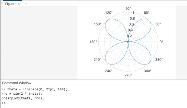
Example 1: Using the syntax polarplot(theta,rho)

theta = linspace(0, 2*pi, 100);
rho = sin(2 * theta);
polarplot(theta, rho);

In this example,

linspace(0, 2*pi, 100) − Creates an array theta with 100 evenly spaced angles between 0 and 2 radians.
sin(2 * theta) − Generates radial values (rho) based on the sine of twice the angle. This could represent a cyclical pattern.
polarplot(theta, rho) − Plots the polar graph using the generated theta and rho values.

Here − Both theta and rho must be either vectors of the same length or matrices of equal size.If matrices are used, the function plots columns of rho against columns of theta.

When you execute the code in matlab command window the output is −

Example 2: Using polarplot(theta, rho, LineSpec)

The code here is −

theta = linspace(0, 2*pi, 100);
rho = sin(2 * theta);
polarplot(theta, rho, '-or');

In this example −

linspace(0, 2*pi, 100) − Creates an array theta with 100 evenly spaced angles between 0 and 2 radians.
sin(2 * theta) − Generates radial values (rho) based on the sine of twice the angle. This could represent a cyclical pattern.
polarplot(theta, rho, '-or') − Plots the polar graph using the generated theta and rho values. The '-or' LineSpec argument indicates a red line (-) with circle markers (o) for each data point.

LineSpec Explanation

'-or' − This LineSpec consists of three parts.
'-' − Specifies a solid line.
'o' − Specifies circle markers at each data point.
'r' − Specifies red color for the line and markers.

By using LineSpec, you can easily customize the appearance of the polar plot, making it more visually appealing and conveying specific information about the data.

When you execute the code in matlab command window the output is −

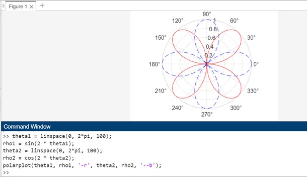
Example 3: Using polarplot(theta1, rho1, ..., thetaN, rhoN)

theta1 = linspace(0, 2*pi, 100);
rho1 = sin(2 * theta1);
theta2 = linspace(0, 2*pi, 100);
rho2 = cos(2 * theta2);
polarplot(theta1, rho1, '-r', theta2, rho2, '--b');

In this example −

linspace(0, 2*pi, 100) − Creates arrays theta1 and theta2 with 100 evenly spaced angles between 0 and 2 radians.
sin(2 * theta1) and cos(2 * theta2) − Generate radial values (rho1 and rho2) based on sine and cosine functions, respectively.
polarplot(theta1, rho1, '-r', theta2, rho2, '--b') − Plots two lines on the polar graph. The first line (theta1, rho1) is a solid red line ('-r'), and the second line (theta2, rho2) is a dashed blue line ('--b').

When you execute the code in matlab command window the output is −

Example 4: Using polarplot(rho)

The code we have for this syntax is −

theta = linspace(0, 2*pi, 100);
rho = sin(2 * theta);
polarplot(rho);

When you execute the code in matlab the output is −

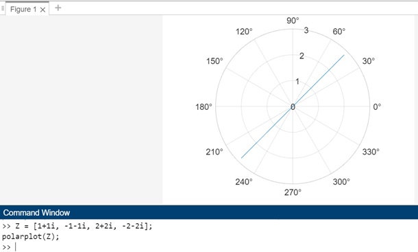
Example 6: Using polarplot(Z)

The code we have by using above syntax is as follows −

Z = [1+1i, -1-1i, 2+2i, -2-2i];
polarplot(Z);

In this example, we create a vector Z containing four complex numbers. We then use polarplot(Z) to plot these complex numbers on a polar plot.

When the code is executed in matlab command window the output is −

Example 7: Using polarplot(Z,LineSpec)

The code we have is −

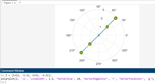
Z = [1+1i, -1-1i, 2+2i, -2-2i];
polarplot(Z, '-o', 'LineWidth', 1.5, 'MarkerSize', 10, 'MarkerEdgeColor', 'r', 'MarkerFaceColor', 'g');

In this example, we use polarplot(Z, '-o') to plot the complex numbers on a polar plot with a solid line ('-') and circle markers ('o'). We then customize the line width ('LineWidth'), marker size ('MarkerSize'), marker edge color ('MarkerEdgeColor'), and marker face color ('MarkerFaceColor') using additional parameters in the LineSpec argument.

When the code is executed in matlab command window the output is −

Plotting Multiple Polar Plot Lines

In MATLAB, polar plots are used to visualize data in polar coordinates, where the angle is represented on the x-axis and the radius (or magnitude) is represented on the y-axis. Multiple line plots can be created on the same polar axis to compare different datasets.

Let us create one example for testing multiple polar plot lines.

theta = linspace(0, 2*pi, 100);
rho1 = sin(2*theta);
rho2 = cos(2*theta);
rho3 = sin(theta);
polarplot(theta, rho1, '-b'); % Plot in blue
hold on;
polarplot(theta, rho2, '--r'); 
polarplot(theta, rho3, '-.g'); 
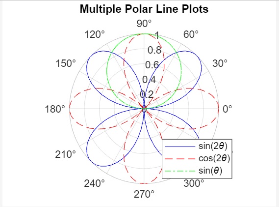
legend('sin(2\theta)', 'cos(2\theta)', 'sin(\theta)', 'Location', 'best');
title('Multiple Polar Line Plots');

The code explanation is as follows −

linspace generates 100 equally spaced values between 0 and 2, which represent the angles for the polar plot.
Three sets of rho values (rho1, rho2, and rho3) are defined using different trigonometric functions of theta. These sets will be plotted as three different line plots on the polar axis.
polarplot() is used to plot the first set of rho values (rho1) with a solid blue line ('-b').
The hold on command is used to prevent the existing plot from being cleared so that more line plots can be added to it.
The second polar plot line with rho values (rho2) is plotted with a dashed red line ('--r').
The third set of rho values (rho3) is plotted with a dash-dot green line ('-.g').
A legend is added to the plot to indicate which line corresponds to which function.Also title is added to the plot to describe its content.

When you execute the code in matlab command window the output is −

Print Page