MATLAB - Laplacian of Gaussian Filter

Quiz

A Gaussian filter is a linear filter used in image processing to blur or smooth images. It is named after the Gaussian function, which is used to define the filter's shape. The Gaussian filter is commonly used to reduce noise and detail in an image, making it more suitable for further processing or analysis.

The Laplacian of Gaussian (LoG) filter is a popular image enhancement and edge detection filter used in image processing. It is a combination of two filters: the Gaussian filter and the Laplacian filter. The Gaussian filter is used to smooth the image and reduce noise, while the Laplacian filter is used to detect edges.

The Laplacian of Gaussian filter is useful for detecting edges at different scales in an image. By varying the standard deviation of the Gaussian filter, you can control the scale at which edges are detected. Smaller standard deviations detect finer details, while larger standard deviations detect broader features.

Let us see a few examples for laplacian of gaussian filter.

Example 1: Using fspecial() Function

The fspecial() function is used to create a Gaussian filter, and then the Laplacian of this Gaussian is computed to create the LoG filter. However, the Laplacian filter expects the Gaussian filter to be of type double.

The code we have is −

% Read the image
img = imread('peppers.jpg');

% Convert the image to grayscale
if size(img, 3) == 3
    img_gray = rgb2gray(img);
else
    img_gray = img;
end

% Create a Gaussian filter
sigma = 2; % Standard deviation of the Gaussian filter
hsize = 2 * ceil(3 * sigma) + 1; % Filter size
gaussian_filter = fspecial('gaussian', hsize, sigma);

% Create a Laplacian of Gaussian filter
log_filter = fspecial('log', hsize, sigma);

% Apply the LoG filter to the image
filtered_img = imfilter(double(img_gray), log_filter, 'conv', 'replicate');

% Display the original and filtered images
subplot(1, 2, 1);
imshow(img_gray);
title('Original Image');

subplot(1, 2, 2);
imshow(uint8(filtered_img));
title('Laplacian of Gaussian Filtered Image');

Let us understand the code in detail −

img = imread('peppers.jpg');

Here it reads the image 'peppers.jpg' from the current directory and stores it in the variable img.

if size(img, 3) == 3
    img_gray = rgb2gray(img);
else
    img_gray = img;
end

If the image is in color (RGB format), it is converted to grayscale using the rgb2gray function. The grayscale image is stored in the variable img_gray. If the image is already in grayscale, it is stored as is.

sigma = 2; % Standard deviation of the Gaussian filter
hsize = 2 * ceil(3 * sigma) + 1; % Filter size
gaussian_filter = fspecial('gaussian', hsize, sigma);

The code above creates the gaussian filter.Here, we define the standard deviation sigma of the Gaussian filter and calculate the filter size hsize based on the standard deviation. We then create the Gaussian filter using the fspecial function with 'gaussian' as the filter type.

log_filter = fspecial('log', hsize, sigma);

We create the Laplacian of Gaussian filter using the fspecial function with 'log' as the filter type. This filter represents the Laplacian of the Gaussian filter, which is used for edge detection.

filtered_img = imfilter(double(img_gray), log_filter, 'conv', 'replicate');

Here the Laplacian of Gaussian filter to the grayscale image img_gray using the imfilter function. The 'conv' option specifies that the filter should be applied using convolution, and the 'replicate' option specifies how the image boundaries should be handled during filtering.

subplot(1, 2, 1);
imshow(img_gray);
title('Original Image');

subplot(1, 2, 2);
imshow(uint8(filtered_img));
title('Laplacian of Gaussian Filtered Image');

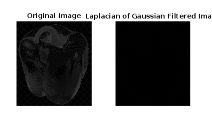
Finally, we display the original grayscale image and the filtered image side by side using the subplot, imshow, and title functions. The filtered image is converted to uint8 format before display.

When the code is executed the output we get is as follows −

Example 2: Image Filtering with Laplacian and LoG Filters

This example shows the application of two different filters, the Laplacian filter and the Laplacian of Gaussian (LoG) filter, to an input image 'peppers.jpg'

The code we have is −

x=imread('peppers.jpg');
figure;
imshow(x);
title('Input Image');
figure;
h=fspecial('laplacian');
filtered_image=imfilter(x,h);
imshow(filtered_image);
title('Output of Laplacian Filter');
figure;
h=fspecial('log');
filtered_image=imfilter(x,h);
imshow(filtered_image);
title('Laplacian Gaussian Filter');

In the example above−

x = imread('peppers.jpg');
figure;
imshow(x);
title('Input Image');

This code reads the image 'peppers.jpg' and displays it using the imshow function. The title function adds a title to the image figure.

h = fspecial('laplacian');
filtered_image = imfilter(x, h);

Here, the Laplacian filter is created using the fspecial function with 'laplacian' as the filter type. The imfilter function is then used to apply this filter to the input image x, resulting in the filtered image filtered_image.

figure;
imshow(filtered_image);
title('Output of Laplacian Filter');

This code displays the filtered image obtained from the Laplacian filter. The title function adds a title to the image figure.

h = fspecial('log');
filtered_image = imfilter(x, h);

Similar to the Laplacian filter, the LoG filter is created using the fspecial function with 'log' as the filter type. The imfilter function is then used to apply this filter to the input image x, resulting in the filtered image filtered_image.

imshow(filtered_image);
title('Laplacian of Gaussian Filter');

This code displays the filtered image obtained from the LoG filter. The title function adds a title to the image figure.

When the code is executed the output we get is −

Print Page