MATLAB - 3D Array Interpolation

Quiz

In MATLAB, 3D array interpolation refers to estimating values within a 3D array at points that are not explicitly defined in the original data. This is useful for creating smoother visualizations or for obtaining values at intermediate points in a three-dimensional space.

Interpolation in a 3D array is similar to interpolation in a 2D array but extends to a third dimension. It allows you to estimate values at points within the array that are not part of the original data set.

Syntax

Vq = interp3(X,Y,Z,V,Xq,Yq,Zq)
Vq = interp3(V,Xq,Yq,Zq)
Vq = interp3(V)
Vq = interp3(V,k)
Vq = interp3(___,method)

Explanation

Detailed explanation of syntax mentioned above −

Vq = interp3(X,Y,Z,V,Xq,Yq,Zq) − Function helps you estimate values in between points of a 3D grid. You provide it with a grid (X, Y, Z) of sample points and their corresponding function values (V). Then, using linear interpolation, it calculates the function values at other points (Xq, Yq, Zq) in the grid. The new values will always fall on the original grid.

Vq = interp3(V,Xq,Yq,Zq) − Assumes a default grid of sample points when you don't specify them. This default grid covers the entire input grid V. It's useful when you want to save memory and don't need to know the exact distances between the points.

Vq = interp3(V) − Returns values interpolated on a finer grid that divides the intervals between sample values once in each dimension.

Vq = interp3(V,k) − Returns values interpolated on a refined grid by repeatedly dividing the intervals k times in each dimension. This creates 2^k-1 interpolated points between sample values.

Vq = interp3(___,method) − Lets you choose a different way to estimate values between sample points by specifying a method like 'linear', 'nearest', 'cubic', 'makima', or 'spline'. The default method is 'linear'.

Examples for 3D Array Interpolation

Here let us try out a few examples on 3d array interpolation using the syntax mentioned above.

Example 1

Following is an example to calculate 3D array interpolation using Vq = interp3(X,Y,Z,V,Xq,Yq,Zq) −

[X, Y, Z] = meshgrid(1:5, 1:5, 1:5);
V = sin(X) .* cos(Y) .* exp(Z);

[Xq, Yq, Zq] = meshgrid(1:0.5:5, 1:0.5:5, 1:0.5:5);

Vq = interp3(X, Y, Z, V, Xq, Yq, Zq);

% Plot original and interpolated data
subplot(1, 2, 1);
slice(X, Y, Z, V, 3, 3, 3);
title('Original Data');

subplot(1, 2, 2);
slice(Xq, Yq, Zq, Vq, 3, 3, 3);
title('Interpolated Data');

In the example above we have −

We first create a 3D grid (X, Y, Z) of sample points using meshgrid().
Then, we define function values V using some mathematical expression.
Next, we create a finer grid (Xq, Yq, Zq) for interpolation.
Using interp3(), we interpolate the function values V at the query points (Xq, Yq, Zq) using linear interpolation.
Finally, we plot both the original and interpolated data using the slice() function to visualize the 3D grids.

When the code is executed in matlab command window the output is −

Example 2

Following is an example to calculate 3D array interpolation using Vq = interp3(V,Xq,Yq,Zq) −

[X, Y, Z] = meshgrid(1:5, 1:5, 1:5);
V = X + Y + Z; % Sample function (sum of coordinates)

[Xq, Yq, Zq] = meshgrid(1:0.5:5, 1:0.5:5, 1:0.5:5);

% Interpolate
Vq = interp3(X, Y, Z, V, Xq, Yq, Zq);

% Plotting
figure;
slice(X, Y, Z, V, [1, 3, 5], [1, 3, 5], [1, 3, 5]); % Original data
hold on;
slice(Xq, Yq, Zq, Vq, [1, 3, 5], [1, 3, 5], [1, 3, 5]); % Interpolated data
hold off;
xlabel('X-axis');
ylabel('Y-axis');
zlabel('Z-axis');
legend('Original Data', 'Interpolated Data');
title('Interpolation in a 3D Grid');

In the example above we have −

We start by creating a 3D grid V using the meshgrid function. This grid represents a simple function where each point's value is the sum of its X, Y, and Z coordinates. This is just a sample function for demonstration purposes.
We then create a finer grid of query points (Xq, Yq, Zq) using meshgrid. These points are where we want to interpolate the values.
Using the interp3 function, we interpolate the values at the query points (Xq, Yq, Zq) based on the values in the original grid (V).
We use the slice function to visualize the original data (V) and the interpolated data (Vq) in the 3D grid. The slice function creates slice planes through the volume data and displays them in a single figure.

On code execution the output we get is as follows −

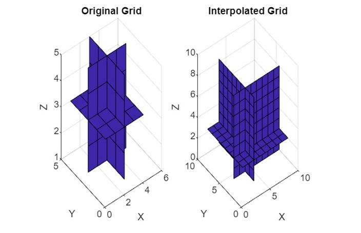
Example 3

Following is an example to calculate 3D array interpolation using Vq = interp3(V) −

V = zeros(5, 5, 5);
V(3, 3, 3) = 1; 

% Perform 3D interpolation
Vq = interp3(V);

% Plotting
figure;
subplot(1, 2, 1);
slice(V, 3, 3, 3); % Original grid
title('Original Grid');
xlabel('X'); ylabel('Y'); zlabel('Z');

subplot(1, 2, 2);
slice(Vq, 3, 3, 3); % Interpolated grid
title('Interpolated Grid');
xlabel('X'); ylabel('Y'); zlabel('Z');

In the example above we have −

We create a 5x5x5 array V with all elements initialized to zero, except for one element at index (3, 3, 3) set to 1.
The interp3(V) function is then called, which interpolates the 3D array V to estimate values in between the existing points.
We use slice to visualize the original and interpolated grids centered at index (3, 3, 3) along each dimension (X, Y, Z). The interpolated grid shows how values are estimated between the points of the original grid.

On code execution the output we get is as follows −

Example 4

Following is an example to calculate 3D array interpolation using Vq = interp3(V,k) −

[X, Y, Z] = meshgrid(1:5, 1:5, 1:5);
V = sin(X) .* cos(Y) .* Z;

k = 2; % Halve the intervals twice in each dimension
Vq = interp3(V, k);

% Plotting
figure;
subplot(1, 2, 1);
slice(V, 3, 3, 3); % Original grid
title('Original Grid');
xlabel('X'); ylabel('Y'); zlabel('Z');

subplot(1, 2, 2);
slice(Vq, 3, 3, 3); % Interpolated grid
title('Interpolated Grid (k=2)');
xlabel('X'); ylabel('Y'); zlabel('Z');

In the example above we have −

We create a 3D array V using meshgrid and fill it with values based on a function of sin, cos, and the meshgrid coordinates.
The interp3(V, k) function is then called with k=2, which means we want to halve the intervals twice in each dimension, resulting in a finer grid.
We use slice to visualize the original and interpolated grids centered at index (3, 3, 3) along each dimension (X, Y, Z). The interpolated grid shows how values are estimated between the points of the original grid with a finer resolution.

On code execution the output we get is as follows −

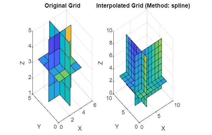
Example 5

Following is an example to calculate 3D array interpolation using Vq = interp3(___,method) spline method −

[X, Y, Z] = meshgrid(1:5, 1:5, 1:5);
V = sin(X) .* cos(Y) .* Z;

Vq = interp3(V, 'spline');

% Plotting
figure;
subplot(1, 2, 1);
slice(V, 3, 3, 3); % Original grid
title('Original Grid');
xlabel('X'); ylabel('Y'); zlabel('Z');

subplot(1, 2, 2);
slice(Vq, 3, 3, 3); % Interpolated grid using 'spline' method
title('Interpolated Grid (Method: spline)');
xlabel('X'); ylabel('Y'); zlabel('Z');

In the example above we have −

We create a 3D array V using meshgrid and fill it with values based on a function of sin, cos, and the meshgrid coordinates.
The interp3(V, 'spline') function is then called, specifying the 'spline' method for interpolation. This method uses spline interpolation to estimate values between the points of the original grid.
We use slice to visualize the original and interpolated grids centered at index (3, 3, 3) along each dimension (X, Y, Z). The 'spline' method provides a smooth interpolation between the points of the original grid.

On code execution the output we get is as follows −

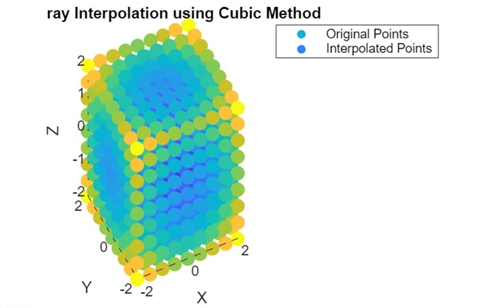
Example 6

Following is an example to calculate 3D array interpolation using cubic method −

[X, Y, Z] = meshgrid(-2:2, -2:2, -2:2);
V = X.^2 + Y.^2 + Z.^2;

% Define the query points
[Xq, Yq, Zq] = meshgrid(-2:0.5:2, -2:0.5:2, -2:0.5:2);

% Perform 3D array interpolation using the cubic method
Vq = interp3(X, Y, Z, V, Xq, Yq, Zq, 'cubic');

% Plot the original and interpolated data
figure;
scatter3(X(:), Y(:), Z(:), 100, V(:), 'filled');
hold on;
scatter3(Xq(:), Yq(:), Zq(:), 100, Vq(:), 'filled');
legend('Original Points', 'Interpolated Points');
title('3D Array Interpolation using Cubic Method');
xlabel('X');
ylabel('Y');
zlabel('Z');

In the example above we have −

We create a 3D array V using meshgrid to represent a 3D function.
Define a new set of query points Xq, Yq, and Zq using meshgrid to specify where we want to interpolate.
Use interp3 with the cubic method to perform the interpolation.
Plot the original points in V and the interpolated points in Vq using scatter3 to visualize the interpolation process.

When the code is executed we get −

Print Page