MATLAB - Add Legend to Axes

Quiz

In MATLAB, a legend is a graphical representation of the data series or elements present in a plot. It helps users understand the meaning of different colors, line styles, or markers used in the plot by providing labels for each element. Legends are particularly useful when a plot contains multiple data series or when distinguishing between different types of data.

By adding a legend to a plot, users can easily identify which data series corresponds to which set of values, making the plot more informative and easier to interpret. Legends can be customized in terms of position, orientation, font size, and other properties to enhance the clarity and aesthetics of the plot.

The legend function is used to create a legend in MATLAB.

Syntax

legend
legend(label1,...,labelN)
legend(labels)
legend(subset,___)
legend(target,___)

Syntax Explanation

legend − A legend in MATLAB is like a key to understand a plot. It shows what each line, color, or symbol in the plot represents. When you plot data in MATLAB, you can give each set of data a name, and the legend will use these names to label the plot. If you don't give a name, MATLAB will label the data as 'data1', 'data2', etc.

The legend is smart and updates itself when you add or remove data from the plot. If there's no plot yet, the legend will be empty. If there are no axes at all, MATLAB will create a set of axes for the legend to go with.

legend(label1,...,labelN) − Function in MATLAB is used to add labels to a plot to explain what each part of the plot represents. You can use it like this: legend('Label1', 'Label2', 'Label3') to label different parts of the plot with 'Label1', 'Label2', and 'Label3'.

legend(labels) − Function in MATLAB is used to add labels to a plot to explain what each part of the plot represents. You can use it like this: legend({'Label1', 'Label2', 'Label3'}) to label different parts of the plot with 'Label1', 'Label2', and 'Label3'.

legend(subset,___) − Function in MATLAB can be used to show only specific items from a plot in the legend. You can do this by providing a vector of graphics objects that represent the items you want to include. This means you can choose which parts of your plot are explained in the legend, showing only the elements you select.

legend(target,___) − Function in MATLAB can be used to create a legend for a specific set of axes or visualization, instead of the one currently active. You can do this by specifying the target axes or visualization as the first input argument to the legend function. This allows you to place the legend wherever you want, regardless of the current plot.

Example 1: Using Legend in the Example

The code we have is.

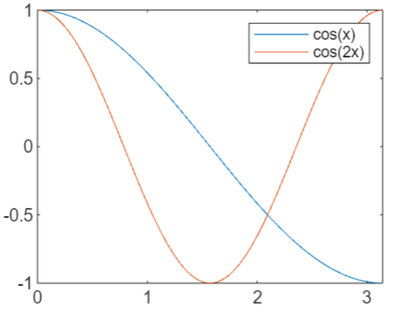
% Create an array of values from 0 to pi
x = linspace(0, pi);

% Calculate y1 = cos(x) and plot it with a label 'cos(x)'
y1 = cos(x);
plot(x, y1, 'DisplayName', 'cos(x)')

% Hold the current plot to add another plot
hold on

% Calculate y2 = cos(2x) and plot it with a label 'cos(2x)'
y2 = cos(2*x);
plot(x, y2, 'DisplayName', 'cos(2x)')

% Release the hold to prevent further plots from being added to the current figure
hold off

% Display the legend with labels for each plot
legend

In the example above −

We create an array x with values ranging from 0 to using the linspace function.We calculate y1 which is the cosine of each value in x, representing cos(x).
We plot y1 with a blue line and label it as 'cos(x)' using the 'DisplayName' parameter in the plot function.We use hold on to keep the current plot active so that we can add another plot.
We calculate y2 which is the cosine of 2*x, representing cos(2x).We plot y2 with a red dashed line and label it as 'cos(2x)'.
We use hold off to release the hold, preventing further plots from being added to the current figure.
Finally, we display the legend using the legend function, which automatically uses the display names ('DisplayName') set in the plot function to label each plot.

The output we have is −

Example 2: Using legend(label1,...,labelN) Syntax

The code we have is

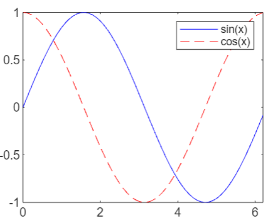
x = 0:0.1:2*pi;
y1 = sin(x);
y2 = cos(x);

plot(x, y1, 'b-', x, y2, 'r--');
legend('sin(x)', 'cos(x)');

In this example, we plot sin(x) and cos(x) and then use the legend function to add a legend to the plot. The legend function takes strings as arguments, which are used as labels for the corresponding data series.

On execution the output we have is −

Example 3: Using Syntax legend(labels)

The code we have is −

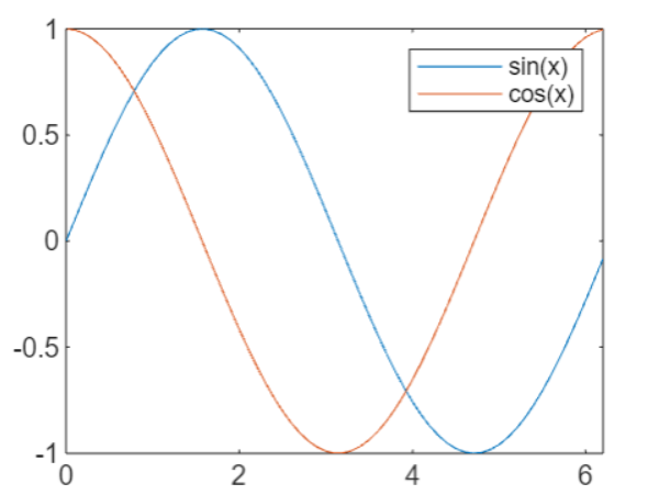
x = 0:0.1:2*pi;
y1 = sin(x);
y2 = cos(x);

plot(x, y1, x, y2);
legend({'sin(x)', 'cos(x)'});

In the example above −

We create a vector x from 0 to 2 with a step size of 0.1.
We calculate the sine and cosine values of x and store them in y1 and y2, respectively.
We plot both y1 and y2 against x.
The legend function is used with a cell array {'sin(x)', 'cos(x)'} as its argument. Each string in the cell array represents a label for the corresponding data series. This syntax allows us to label different parts of the plot with 'sin(x)' and 'cos(x)'.

On execution the output we have is −

Example 4: Using Syntax legend(subset,___)

The code we have is as follows −

x = linspace(0, pi);

y1 = cos(x);
p1 = plot(x, y1);

hold on

y2 = cos(2*x);
plot(x, y2);

y3 = cos(3*x);
p3 = plot(x, y3);

% Release the hold to prevent further plots from being added to the current figure
hold off

% Display the legend with labels for the first and third plots
legend([p1, p3], {'First', 'Third'})

In the example above −

We create an array x with values ranging from 0 to using the linspace function.
We calculate y1 which is the cosine of each value in x, representing cos(x), and plot it, saving the plot handle as p1.
We use hold on to keep the current plot active so that we can add more plots.
We calculate y2 which is the cosine of 2*x, representing cos(2x), and plot it (but don't save the plot handle).
We calculate y3 which is the cosine of 3*x, representing cos(3x), and plot it, saving the plot handle as p3.
We use hold off to release the hold, preventing further plots from being added to the current figure.
Finally, we display the legend using the legend function, specifying the plot handles [p1, p3] to include only the first and third plots in the legend, and providing labels 'First' and 'Third' for them.

The output is −

Example 5: Using Syntax legend(target,___)

The code we have is −

figure;
ax = gca;

x = 0:0.1:2*pi;
y1 = sin(x);
y2 = cos(x);
plot(ax, x, y1, x, y2);

title(ax, 'Trigonometric Functions');
xlabel(ax, 'x');
ylabel(ax, 'y');

legend(ax, {'sin(x)', 'cos(x)'}, 'Location', 'best');

In the example above −

We create a new figure and get the current axes (ax) using gca.
We plot the sine and cosine functions on the specified axes ax.
We set the title and labels for the axes to provide context for the plot.
The legend function is used with the specified axes ax as the first argument. This tells MATLAB to create the legend for the specified axes, not the current one.
The legend is created with labels 'sin(x)' and 'cos(x)' for the respective plots, and the 'Location', 'best' argument is used to place the legend in the best location on the axes.Using the legend(target,___) syntax allows you to create legends for specific axes, which is useful when you have multiple plots or figures and want to control where the legend is displayed.

The output is −

Print Page