MATLAB - Plot Spectrogram

Quiz

Spectrograms are a powerful tool used in signal processing and audio analysis to visualize the frequency content of a signal over time. MATLAB provides a simple and efficient way to plot spectrograms using the spectrogram function, which is part of the Signal Processing Toolbox.

What is Spectrogram?

A spectrogram is a visual representation of the spectrum of frequencies of a signal as it varies with time. It's a 2D plot where the x-axis represents time, the y-axis represents frequency, and the color or intensity represents the magnitude of the frequencies at each point in time.

Spectrograms are commonly used in signal processing, music analysis, and speech processing to analyze the frequency content of a signal over time. They can reveal important information about the underlying structure of a signal, such as the presence of certain frequencies or how they change over time.

In audio processing, spectrograms are often used to visualize the frequency components of a sound signal, allowing users to identify patterns, trends, and anomalies in the signal. They are also used in various other fields, such as sonar, radar, and medical imaging, where the analysis of signals in the frequency domain is important.

Understanding Spectrogram Function

The spectrogram function in MATLAB computes the spectrogram of a signal and plots it as a surface or image. The syntax is as follows −

Syntax

s = spectrogram(x)
s = spectrogram(x,window)
s = spectrogram(x,window,noverlap)
s = spectrogram(x,window,noverlap,nfft)

The detailed explanation of the syntax is as follows −

s = spectrogram(x) − The spectrogram function in MATLAB calculates the Short-Time Fourier Transform (STFT) of a given input signal x. This means it breaks down the signal into short segments and analyzes the frequency content of each segment. The result, s, is a matrix where each column represents the frequency content of a specific segment of the signal. The squared magnitude of s gives us a visual representation called the spectrogram, which shows how the signal's frequency content changes over time.

s = spectrogram(x,window) − The window parameter to split the input signal x into segments and applies a windowing function to each segment. This helps in analyzing the signal's frequency content over time with better accuracy.

s = spectrogram(x,window,noverlap) − noverlap samples of overlap between adjacent segments when dividing the input signal x into segments using the specified window. This overlapping helps in capturing more detailed information about the signal's frequency content over time.

s = spectrogram(x,window,noverlap,nfft) − nfft sampling points to calculate the discrete Fourier transform (DFT) of each segment of the input signal x. This helps in analyzing the signal's frequency content with more detail and accuracy.

Examples of MATLAB Spectrogram

Here are a few examples of how to use spectrogram in MATLAB −

Example 1: Using s = spectrogram(x)

The code is as follows −

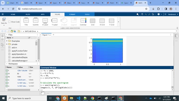
fs = 1000;
t = 0:1/fs:1;
f1 = 50;
x = sin(2*pi*f1*t);

% Calculate the spectrogram
s = spectrogram(x);
imagesc(t, f, 10*log10(abs(s)))

In above example

fs = 1000; − This sets the sampling frequency of the signal to 1000 Hz.
t = 0:1/fs:2; − This creates a time vector t from 0 to 2 seconds with a sampling interval of 1/fs seconds.
f1 = 50; − This is the frequency of the sinusoid in the signal.
x = sin(2*pi*f1*t); − This generates the test signal, which is a sinusoid with frequency f1.
spectrogram(x) − This calculates the spectrogram of the signal x. The function returns three outputs: s (the spectrogram values), f (the frequency vector), and t (the time vector).
imagesc(t, f, 10*log10(abs(s))) − This plots the spectrogram using the imagesc function. The 10*log10(abs(s)) part converts the spectrogram values to dB scale for better visualization.

When the code is executed in matlab command window the output is −

Example 2: Plot Spectrogram of Sum of two Sine Waves

The code we have is as follows −

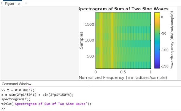
t = 0:0.001:2;
z = sin(2*pi*50*t) + sin(2*pi*150*t);
spectrogram(z);
title('Spectrogram of Sum of Two Sine Waves');

In this example, the signal z is created by summing two sine waves with frequencies of 50 Hz and 150 Hz, respectively. The spectrogram will show the frequency content of this combined signal over time.

When you execute the output is as follows −

Example 3: Plot Spectrogram Quadratic Signal

The code we have is as follows −

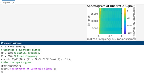
t = 0:0.0001:2;
% Generate a quadratic signal
f0 = 100; % Initial frequency
f1 = 200; % Final frequency
x = sin(2*pi*(f0 + (f1 - f0)*t.^2/(2*max(t))) .* t);
% Plot the spectrogram
spectrogram(x);
title('Spectrogram of Quadratic Signal');

In this example, the signal x is generated using a quadratic function to modulate the frequency of a sine wave over time. The spectrogram will show the frequency content of this quadratic signal over time.

When executed in matlab command window the output is −

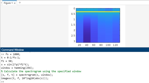
Example 4: Using s = spectrogram(x,window)

The code is as follows −

fs = 1000; 
t = 0:1/fs:1;
f1 = 50;
x = sin(2*pi*f1*t);
window = hamming(256);
% Calculate the spectrogram using the specified window
[s, f, t] = spectrogram(x, window);
imagesc(t, f, 10*log10(abs(s)));

In above example we have −

fs = 1000; − This sets the sampling frequency of the signal to 1000 Hz.

t = 0:1/fs:1; − This creates a time vector t from 0 to 1 second with a sampling interval of 1/fs seconds.

f1 = 50; − This is the frequency of the sinusoid in the signal.

x = sin(2*pi*f1*t); − This generates the test signal, which is a sinusoid with frequency f1.

window = hamming(256); − This defines the windowing function as a Hamming window of length 256. The windowing function is applied to each segment of the signal before computing the spectrogram.

spectrogram(x, window) − This calculates the spectrogram of the signal x using the specified window. The function returns three outputs: s (the spectrogram values), f (the frequency vector), and t (the time vector).

imagesc(t, f, 10*log10(abs(s))) − This plots the spectrogram using the imagesc function. The 10*log10(abs(s)) part converts the spectrogram values to dB scale for better visualization.

When you execute the code in matlab command window the output is −

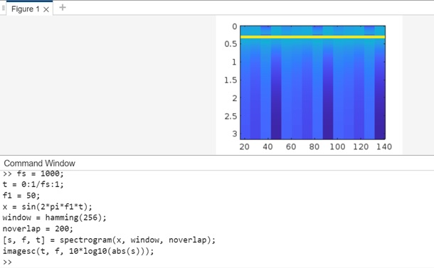
Example 5: Using s = spectrogram(x,window,noverlap)

The code we have is as follows −

fs = 1000;
t = 0:1/fs:1;
f1 = 50;
x = sin(2*pi*f1*t);
window = hamming(256);
noverlap = 200;
[s, f, t] = spectrogram(x, window, noverlap);
imagesc(t, f, 10*log10(abs(s)));

In the above code we have −

fs = 1000; − This sets the sampling frequency of the signal to 1000 Hz.
t = 0:1/fs:1; − This creates a time vector t from 0 to 1 second with a sampling interval of 1/fs seconds.
f1 = 50; − This is the frequency of the sinusoid in the signal.
x = sin(2*pi*f1*t); − This generates the test signal, which is a sinusoid with frequency f1.
window = hamming(256); − This defines the windowing function as a Hamming window of length 256. The windowing function is applied to each segment of the signal before computing the spectrogram.
noverlap = 200; − This sets the number of overlapping samples between adjacent segments.
spectrogram(x, window, noverlap) − This calculates the spectrogram of the signal x using the specified window and noverlap. The function returns three outputs: s (the spectrogram values), f (the frequency vector), and t (the time vector).
imagesc(t, f, 10*log10(abs(s))) − This plots the spectrogram using the imagesc function. The 10*log10(abs(s)) part converts the spectrogram values to dB scale for better visualization.

When you execute the code in matlab command window the output is −

Example 6: Using s = spectrogram(x,window,noverlap,nfft)

The code we have is as follows −

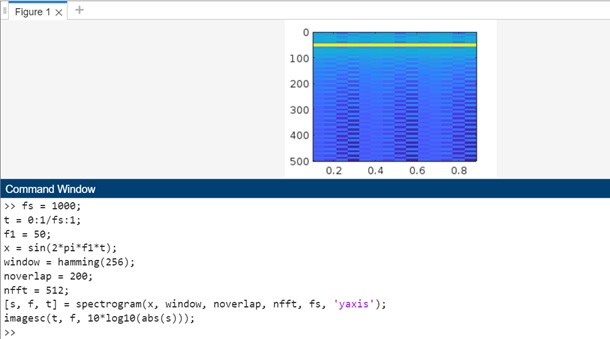
fs = 1000;
t = 0:1/fs:1;
f1 = 50;
x = sin(2*pi*f1*t);
window = hamming(256);
noverlap = 200;
nfft = 512;
[s, f, t] = spectrogram(x, window, noverlap, nfft, fs, 'yaxis');
imagesc(t, f, 10*log10(abs(s)));

In above we have −

fs = 1000; − This sets the sampling frequency of the signal to 1000 Hz.
t = 0:1/fs:1; − This creates a time vector t from 0 to 1 second with a sampling interval of 1/fs seconds.
f1 = 50; − This is the frequency of the sinusoid in the signal.
x = sin(2*pi*f1*t); − This generates the test signal, which is a sinusoid with frequency f1.
window = hamming(256); − This defines the windowing function as a Hamming window of length 256. The windowing function is applied to each segment of the signal before computing the spectrogram.
noverlap = 200; − This sets the number of overlapping samples between adjacent segments.
nfft = 512; − This sets the number of FFT points used to calculate the discrete Fourier transform (DFT) of each segment. More FFT points can provide a higher frequency resolution in the spectrogram.
spectrogram(x, window, noverlap, nfft, fs, 'yaxis') − This calculates the spectrogram of the signal x using the specified window, noverlap, and nfft. The 'yaxis' argument specifies the y-axis scaling as frequency in Hz.
imagesc(t, f, 10*log10(abs(s))) − This plots the spectrogram using the imagesc function. The 10*log10(abs(s)) part converts the spectrogram values to dB scale for better visualization.

When you execute the code the output is as follows −

Print Page