MATLAB - Fast Fourier Transform

Quiz

The Fast Fourier Transform (FFT) is a widely used mathematical algorithm in signal processing and other fields for efficiently computing the Discrete Fourier Transform (DFT) and its inverse. The DFT converts a signal from its original domain (typically time or space) to a representation in the frequency domain.

The main advantage of the Fast Fourier Transform over the standard DFT is its speed. While the standard DFT algorithm has a computational complexity of O(N^2), where N is the number of samples in the signal, the FFT reduces this to O(N log N), making it much faster for large datasets.

Working with Fast Fourier Transform Using fft() Function in Matlab

The fft() function in MATLAB is used to compute the Fast Fourier Transform (FFT) of a signal. It takes a vector representing a signal in the time domain as input and returns a vector representing the signal in the frequency domain.

Syntax

Y = fft(X)
Y = fft(X,n)
Y = fft(X,n,dim)

Syntax Explanation

Y = fft(X) − Function in MATLAB calculates the Fourier transform of a signal. If you provide a vector, it computes the transform for that vector. If you provide a matrix, it calculates the transform for each column of the matrix. For multidimensional arrays, it treats the values along the first non-singleton dimension as vectors and computes the transform for each vector.

Y = fft(X,n) − The fft() function in MATLAB can calculate a specific length Fourier transform called the n-point DFT.

If you provide a vector X that is shorter than n, it adds zeros to the end of X to make it length n. If X is longer than n, it cuts off the extra values.

If X is a matrix, it processes each column as if it were a vector.

For multidimensional arrays, it treats the first non-singleton dimension as if it were a vector.

Y = fft(X,n,dim) − The fft() function in MATLAB can calculate the Fourier transform along a specific dimension of a matrix or multidimensional array.For example, if you have a matrix X and you use fft(X,n,2), it will calculate the n-point Fourier transform of each row of the matrix.

Let us see a few examples for syntaxes we explained above.

Example 1: Visualize the Fourier transform of a Simple Input Signal

The code we have is as follows −

x = [0, 1, 0, -1];
Y = fft(x);

% Plotting
figure;

subplot(2,1,1);
stem(x);
title('Input Signal');
xlabel('Time');
ylabel('Amplitude');

subplot(2,1,2);
stem(abs(Y));
title('Magnitude of Fourier Transform');
xlabel('Frequency');
ylabel('Magnitude');

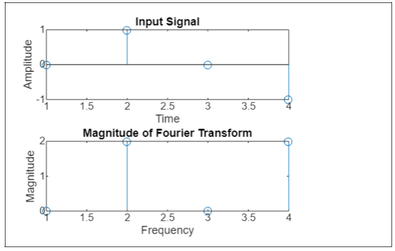
In this example, we have a simple input signal x represented by a vector [0, 1, 0, -1].

The fft(x) function calculates the discrete Fourier transform (DFT) of the input signal x using the fast Fourier transform (FFT) algorithm. The result is stored in the variable Y.

After computing the Fourier transform, we create a figure to plot the input signal and its Fourier transform for visualization purposes.

In the first subplot (subplot(2,1,1)), we use the stem() function to plot the input signal x in the time domain. The x-axis represents time, and the y-axis represents the amplitude of the signal.

In the second subplot (subplot(2,1,2)), we use the abs() function to calculate the magnitude of the Fourier transform Y since the Fourier transform can have complex values. We then use stem() to plot the magnitude of the Fourier transform. Here, the x-axis represents frequency, and the y-axis represents the magnitude of the Fourier coefficients.

The output on execution is as follows −

Example 2: Fast Fourier Transform Using Matrix

The code we have is −

X = [1, 2, 3; 4, 5, 6; 7, 8, 9];
Y = fft(X);

% Plotting
figure;

subplot(2,1,1);
stem(X(:));
title('Input Matrix (Vectorized)');
xlabel('Index');
ylabel('Value');

subplot(2,1,2);
stem(abs(Y(:)));
title('Magnitude of Fourier Transform (Vectorized)');
xlabel('Frequency Index');
ylabel('Magnitude');

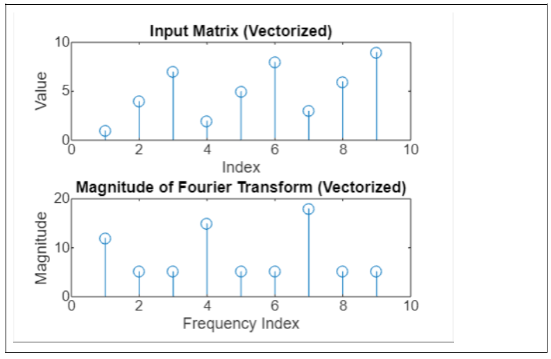
In this example, the first subplot shows the input matrix X (vectorized) with the matrix elements along the x-axis and their values on the y-axis. The second subplot shows the magnitude of the Fourier transform Y of the matrix (vectorized), with the frequency index on the x-axis and the magnitude of the Fourier coefficients on the y-axis.

On execution the output is as follows −

Example 3: Fast Fourier Transform Using Syntax Y = fft(x,n)

The code we have is as follows −

x = [0, 1, 0, -1];
n = 8; % Desired length of the Fourier transform
Y = fft(x, n);

% Plotting
figure;

subplot(2,1,1);
stem(x);
title('Input Signal');
xlabel('Time');
ylabel('Amplitude');

subplot(2,1,2);
stem(abs(Y));
title('Magnitude of Fourier Transform (n-point DFT)');
xlabel('Frequency');
ylabel('Magnitude');

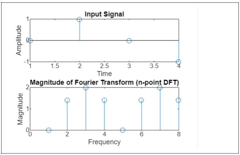
In this example, we have a vector x representing our input signal. We want to compute an 8-point discrete Fourier transform (DFT) of x using the syntax Y = fft(x, n).

Since the length of x is 4, which is shorter than n (8), MATLAB adds zeros to the end of x to make it length 8 before computing the Fourier transform.

After computing the Fourier transform, we create a figure to plot the input signal and its Fourier transform for visualization.

In the first subplot (subplot(2,1,1)), we use the stem() function to plot the input signal x in the time domain. The x-axis represents time, and the y-axis represents the amplitude of the signal.

On execution the output we have is −

Example 4: Fourier Transform of Each Row of a Matrix

The code we have is as follows −

X = [1, 2, 3; 4, 5, 6];

% Compute the 4-point Fourier transform of each row
n = 4; % Desired length of the Fourier transform
Y = fft(X, n, 2);

% Display the result
disp('Matrix X:');
disp(X);
disp('Fourier Transform of Each Row (n-point DFT):');
disp(Y);

In this code, we first define a matrix X with two rows, where each row represents a different signal. We then compute the 4-point Fourier transform of each row of X using fft(X, n, 2), where n is the desired length of the Fourier transform. Finally, we display the original matrix X and the Fourier transform of each row.

When the code the executed the output is −

X = [1, 2, 3; 4, 5, 6];

% Compute the 4-point Fourier transform of each row
n = 4; % Desired length of the Fourier transform
Y = fft(X, n, 2);

% Display the result
disp('Matrix X:');
disp(X);
disp('Fourier Transform of Each Row (n-point DFT):');
disp(Y);

Matrix X:
     1     2     3
     4     5     6

Fourier Transform of Each Row (n-point DFT):
   6.0000 + 0.0000i  -2.0000 - 2.0000i   2.0000 + 0.0000i  -2.0000 + 2.0000i
  15.0000 + 0.0000i  -2.0000 - 5.0000i   5.0000 + 0.0000i  -2.0000 + 5.0000i

Print Page