MATLAB - Histograms

---

---

Histograms are graphical representations that display the distribution of numerical data. MATLAB provides a convenient function, histogram, to create histograms, allowing users to visualize the frequency or probability distribution of a dataset across different intervals or bins.

Syntax

histogram(X)
histogram(X,nbins)
histogram(X,edges)
histogram('BinEdges',edges,'BinCounts',counts)
histogram(C)
histogram(C,Categories)
histogram('Categories',Categories,'BinCounts',counts)

Detailed explanation of syntax −

histogram(X) − The 'histogram(X)' function generates a histogram plot based on the data in X. This function employs an automated binning method that produces bins of equal width, designed to span the range of values within X and uncover the inherent distribution pattern. The output is presented as rectangular bars, with the height of each bar representing the count of elements falling within the corresponding bin.

histogram(X,nbins) − The 'histogram(X, nbins)' function allows you to define the quantity of bins to be used in the histogram.

histogram(X,edges) − The 'histogram(X, edges)' function organizes the data in X into bins determined by the edges specified within a vector.

histogram('BinEdges',edges,'BinCounts',counts) − The 'histogram('BinEdges', edges, 'BinCounts', counts)' function directly plots the provided bin counts without performing any binning of the data.

histogram(C) − The 'histogram(C)' function generates a histogram displaying a bar for every category present in the categorical array C.

histogram(C,Categories) − The 'histogram(C, Categories)' function specifically plots a selection of categories from the categorical array C.

histogram('Categories',Categories,'BinCounts',counts) − The 'histogram('Categories', Categories, 'BinCounts', counts)' function allows manual specification of categories along with their respective bin counts. The histogram then plots the provided bin counts without performing any data binning.

Histogram Properties

The Histogram function returns as an object.

Properties of histograms regulate their appearance and functionality. Altering these property values allows for adjustments to various histogram aspects. Utilize dot notation to access specific object properties −

h = histogram(randn(10,1));
c = h.BinWidth;
h.BinWidth = 2;

Bins in Histogram

In a histogram, bins represent intervals into which the data is divided. These intervals cover the range of the data and are used to count the frequency of observations falling within each interval. Essentially, bins define the boundaries that separate different ranges of data values, and the height of the bars in the histogram corresponds to the frequency or count of data points falling within each bin. Adjusting the number or width of bins can impact how the distribution is visualized, potentially revealing more granularity or smoothing out the representation of the data.

Number of Bins

The number of bins is denoted by a positive integer. When NumBins isn't specified, the histogram function automatically determines the suitable bin count from the provided data. If you use NumBins alongside BinMethod, BinWidth, or BinEdges, the histogram function only considers the last parameter.

Width of Bins

The bin width represents a positive scalar value. When you define BinWidth, the histogram can utilize a maximum of 65,536 bins (or 216). If the specified bin width demands more bins, the histogram adjusts to a larger bin width, accommodating the maximum bin count. For datetime and duration data, BinWidth can be a scalar duration or calendar duration. When you use BinWidth along with BinMethod, NumBins, or BinEdges, the histogram function only considers the last parameter.

Example − histogram(X,'BinWidth',5) uses bins with a width of 5 units.

Edges of Bins

Bin edges are defined by a numeric vector, where the initial element indicates the starting edge of the first bin, and the final element denotes the ending edge of the last bin. The final edge is considered only for the last bin. In the absence of specified bin edges, the histogram function autonomously computes these edges. If you use BinEdges alongside BinMethod, BinWidth, NumBins, or BinLimits, the histogram function prioritizes BinEdges, and it must be the last parameter provided.

Bin Limits

Bin limits are defined by a two-element vector, [bmin, bmax], where the initial value signifies the starting edge of the first bin and the subsequent value signifies the concluding edge of the last bin. Utilizing these limits involves computing only the data falling inclusively within these bin limits, indicated by X>=bmin & X<=bmax.

Example − histogram(X,'BinLimits',[1,10]) bins only the values in X that lie between 1 and 10, including both boundaries.

Categories in Histogram

In MATLAB, when using the histogram function with categorical data, "Categories" refer to the distinct groups or labels within the categorical array that you want to visualize. When creating a histogram for categorical data, each unique category will have its own bar, and the height of the bar represents the frequency or count of occurrences of that particular category in the dataset.

Categories Included in Histogram

Categories represented in the histogram are defined by a cell array of character vectors, a categorical array, a string array, or a pattern scalar.

Example − h = histogram(C,{'Large','Small'}) creates a histogram displaying only the categorical data associated with the categories 'Large' and 'Small'.

Creating a Basic Histogram

The histogram function in MATLAB generates a histogram. Here's a simple example −

Example 1: Creating Basic Histogram

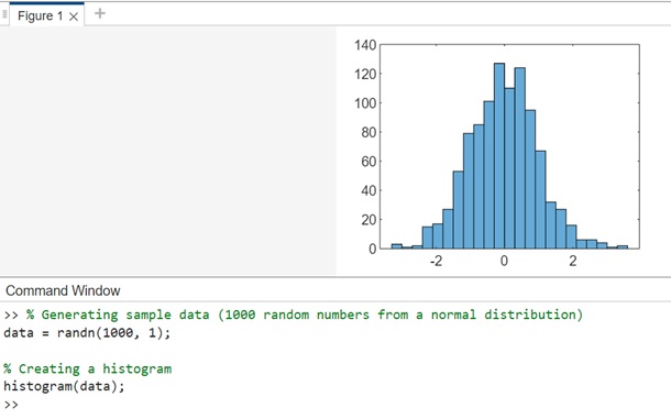
The code generates a histogram from 1000 random numbers sampled from a standard normal distribution (randn). The histogram function automatically determines the appropriate number of bins based on the data.

% Generating sample data (1000 random numbers from a normal distribution)
data = randn(1000, 1);

% Creating a histogram
histogram(data);

When you execute the same in matlab command window the output is −

Let us work on another similar example as shown below −

Example 2: Using Histogram Object to Find Histogram Bins

The code will produce a histogram from a set of 5,000 random numbers. The histogram function automatically selects an optimal number of bins to encompass the range of values in x, effectively illustrating the distribution's form.

x = randn(5000,1);
h = histogram(x)

On execution in matlab command window the output is −

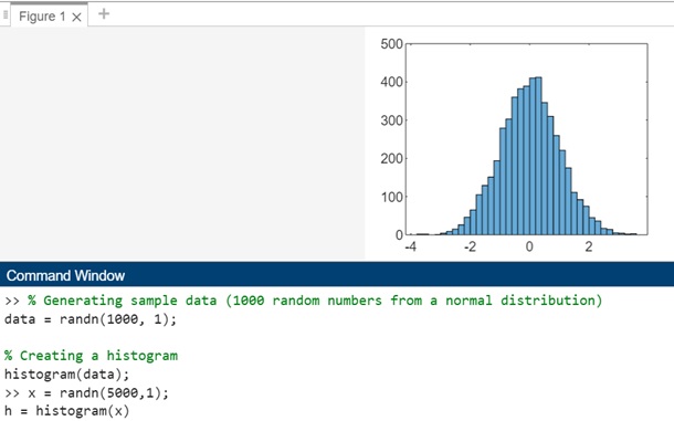
If you designate an output for the histogram function, it provides a histogram object. This object enables the examination of histogram properties, such as bin count or bin width.

The histogram object with the methods and properties can be seen as shown below −

>> x = randn(5000,1);
h = histogram(x)


h = 

  Histogram with properties:

             Data: [5000x1 double]
           Values: [2 2 0 1 4 9 15 26 46 65 105 129 151 194 279 303 360 382 389 410 412 346 310 260 221 175 111 ... ] (1x37 double)
          NumBins: 37
         BinEdges: [-3.8000 -3.6000 -3.4000 -3.2000 -3 -2.8000 -2.6000 -2.4000 -2.2000 -2 -1.8000 -1.6000 ... ] (1x38 double)
         BinWidth: 0.2000
        BinLimits: [-3.8000 3.6000]
    Normalization: 'count'
        FaceColor: 'auto'
        EdgeColor: [0 0 0]

  Show all properties

            Annotation: [1x1 matlab.graphics.eventdata.Annotation]
          BeingDeleted: off
             BinCounts: [2 2 0 1 4 9 15 26 46 65 105 129 151 194 279 303 360 382 389 410 412 346 310 260 ... ] (1x37 double)
         BinCountsMode: 'auto'
              BinEdges: [-3.8000 -3.6000 -3.4000 -3.2000 -3 -2.8000 -2.6000 -2.4000 -2.2000 -2 -1.8000 ... ] (1x38 double)
             BinLimits: [-3.8000 3.6000]
         BinLimitsMode: 'auto'
             BinMethod: 'auto'
              BinWidth: 0.2000
            BusyAction: 'queue'
         ButtonDownFcn: ''
              Children: [0x0 GraphicsPlaceholder]
           ContextMenu: [0x0 GraphicsPlaceholder]
             CreateFcn: ''
                  Data: [5000x1 double]
       DataTipTemplate: [1x1 matlab.graphics.datatip.DataTipTemplate]
             DeleteFcn: ''
           DisplayName: 'x'
          DisplayStyle: 'bar'
             EdgeAlpha: 1
             EdgeColor: [0 0 0]
             FaceAlpha: 0.6000
             FaceColor: 'auto'
      HandleVisibility: 'on'
               HitTest: on
         Interruptible: on
             LineStyle: '-'
             LineWidth: 0.5000
         Normalization: 'count'
               NumBins: 37
           Orientation: 'vertical'
                Parent: [1x1 Axes]
         PickableParts: 'visible'
              Selected: off
    SelectionHighlight: on
           SeriesIndex: 1
                   Tag: ''
                  Type: 'histogram'
              UserData: []
                Values: [2 2 0 1 4 9 15 26 46 65 105 129 151 194 279 303 360 382 389 410 412 346 310 260 ... ] (1x37 double)
               Visible: on

To find the number of histogram bins, you can do as follows −

nbins = h.NumBins

In matlab command window the execution looks as follows −

>> nbins = h.NumBins

nbins =

    37

>> 

Example 3

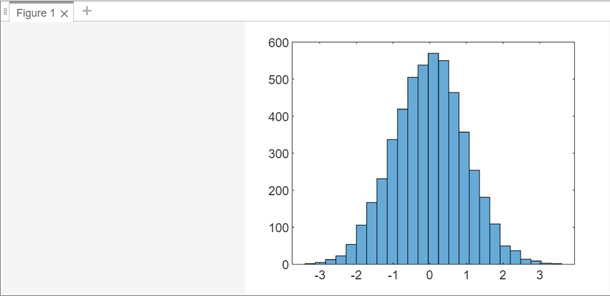
Let us plot a histogram of 5,000 random numbers sorted into 25 equally spaced bins.

x = randn(5000,1);
nbins = 25;
h = histogram(x,nbins)

On execution the output is as follows −

Let us find the bin counts using the code shown below −

counts = h.Values

On execution in matlab command window the output is −

>> counts = h.Values

counts =

  Columns 1 through 21

     2     5    13    23    54   106   167   231   337   419   505   538   570   550   464   357   254   181   109    50    37

  Columns 22 through 25

    14     9     3     2

>>

Example 4: Plot Categorical Histogram

In this example will generate a categorical vector depicting votes. The categories within the vector are 'yes', 'no', or 'undecided'.

A = [0 0 1 1 1 0 0 0 0 NaN NaN 1 0 0 0 1 0 1 0 1 0 0 0 1 1 1 1];
C = categorical(A,[1 0 NaN],{'yes','no','undecided'})

On execution in matlab command window the output is −

>> A = [0 0 1 1 1 0 0 0 0 NaN NaN 1 0 0 0 1 0 1 0 1 0 0 0 1 1 1 1];
C = categorical(A,[1 0 NaN],{'yes','no','undecided'})

C = 

  1x27 categorical array

  Columns 1 through 13

     no      no      yes      yes      yes      no      no      no      no      undecided      undecided      yes      no 

  Columns 14 through 27

     no      no      yes      no      yes      no      yes      no      no      no      yes      yes      yes      yes 

>> 

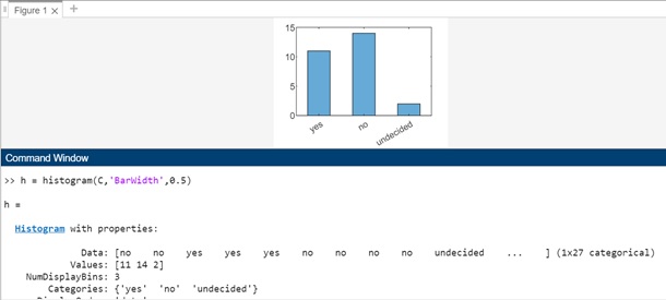
Using the categorical data let us plot a categorical histogram of the votes, using a relative bar width of 0.5.