MATLAB - Plot Expression or Function

Quiz

MATLAB provides powerful tools for visualizing mathematical expressions or functions. You can plot a wide range of functions, from simple linear equations to complex mathematical expressions, and visualize them in 2D or 3D space. This capability is particularly useful for engineers, scientists, and mathematicians who need to analyze and understand the behavior of mathematical functions.

Plotting of expression or function can be done using the following methods in matlab.

fplot() for 2D plotting
fplot3() for 3D plotting

Using fplot() in Matlab

The fplot() function in MATLAB is used to plot a function of one variable over a specified range. It is particularly useful for visualizing mathematical functions and expressions.

Syntax

fplot(f)
fplot(f,xinterval)
fplot(funx,funy)
fplot(funx,funy,tinterval)
fplot(___,LineSpec)
fplot(___,Name,Value)
fplot(ax,___)

Let us understand the syntax in detail.

fplot(f) − Function displays the graph of the function y = f(x) over the default interval [-5 5] for x.

fplot(f,xinterval) − Function plots the graph over a specified interval. The interval should be specified as a two-element vector in the form [xmin xmax].

fplot(funx,funy) − Function displays the curve defined by the parametric equations x = funx(t) and y = funy(t) over the default interval [-5 5] for t.

fplot(funx,funy,tinterval) − The fplot(funx, funy, tinterval) function plots the parametric curve defined by x = funx(t) and y = funy(t) over a specified interval. The interval should be specified as a two-element vector in the form [tmin tmax].

fplot(___,LineSpec) − The fplot(___, LineSpec) option allows you to specify the line style, marker symbol, and line color for the plot. For instance, using '-r' will plot a red line. This option can be used after any of the input argument combinations in the previous syntaxes.

fplot(___,Name,Value) − Using fplot(___, Name, Value) allows you to specify line properties using one or more name-value pair arguments. For example, 'LineWidth', 2 specifies a line width of 2 points. This option can be used after any of the input argument combinations in the previous syntaxes.

fplot(ax,___) − Function plots the graph into the axes specified by ax instead of the current axes (gca). The axes should be specified as the first input argument.

Let us execute a few examples for each of the syntax we have listed above.

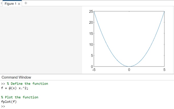
Example 1: Using fplot(f)

Consider we want to plot for the function y = x²

Using the function fplot().

% Define the function
f = @(x) x.^2;

% Plot the function
fplot(f)

When you execute the above code in matlab command window the output is −

Example 2: Using fplot(f,xinterval)

Let's say we want to plot the function y = x³ over the interval [-2, 2].

The code we have is −

% Define the function
f = @(x) x.^3;

% Specify the interval
xinterval = [-2, 2];

% Plot the function over the specified interval
fplot(f, xinterval)

In this example, we first define the function y = x³ using an anonymous function f = @(x) x.^3. We then specify the interval as xinterval = [-2, 2]. The fplot(f, xinterval) function plots this function over the specified interval [-2, 2] for x. Finally, we add a title and labels to the plot for better understanding.

When you execute the code the output is −

Example 3: Using fplot(funx,funy)

Let's say we want to plot a circle using parametric equations −

x=cos(t)

y=sin(t)

% Define the parametric equations for a circle
funx = @(t) cos(t);
funy = @(t) sin(t);

% Plot the circle
fplot(funx, funy)

In this example, we define the parametric equations for a circle using anonymous functions funx = @(t) cos(t) and funy = @(t) sin(t). The fplot(funx, funy) function then plots the circle defined by these parametric equations over the default interval [-5 5] for t.

When you execute the code the output is −

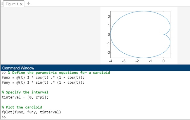
Example 4: Using fplot(funx,funy,tinterval)

Let's say we want to plot a cardioid using parametric equations −

x=2cos(t)(1cos(t))

y=2sin(t)(1cos(t))

over the interval [0,2]

% Define the parametric equations for a cardioid
funx = @(t) 2 * cos(t) .* (1 - cos(t));
funy = @(t) 2 * sin(t) .* (1 - cos(t));

% Specify the interval
tinterval = [0, 2*pi];

% Plot the cardioid
fplot(funx, funy, tinterval)

In this example, we define the parametric equations for a cardioid using anonymous functions funx and funy. We then specify the interval tinterval = [0, 2*pi] for the parameter t. The fplot(funx, funy, tinterval) function then plots the cardioid over this specified interval.

When the code is executed the output is −

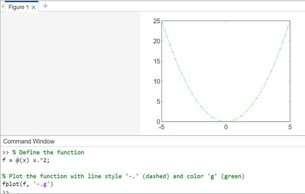
Example 5: Using fplot(___,LineSpec)

Let's say we want to plot the function y = x² using a dashed green line.

% Define the function
f = @(x) x.^2;

% Plot the function with line style '-.' (dashed) and color 'g' (green)
fplot(f, '-.g')

In this example, we use the '-.' LineSpec to specify a dashed line ('-') with a marker ('.') and color ('g' for green). The fplot(f, '-.g') function then plots the function y = x² using the specified line style, marker, and color.

When you execute the code the output is −

Example 6: Using fplot(___,Name,Value)

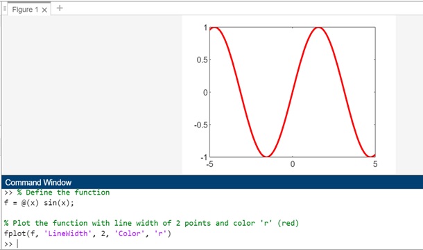
Let's say we want to plot the function y=sin(x) with a thicker red line.

% Define the function
f = @(x) sin(x);

% Plot the function with line width of 2 points and color 'r' (red)
fplot(f, 'LineWidth', 2, 'Color', 'r')

In this example, we use the 'LineWidth' name-value pair argument to specify a line width of 2 points, and the 'Color' name-value pair argument to specify the color red ('r'). The fplot(f, 'LineWidth', 2, 'Color', 'r') function then plots the function y=sin(x) using the specified line width and color.

When you execute the code the output is −

Example 7: Using fplot(ax,___)

Let's say we want to plot the function y = x2 into a specific set of axes instead of the default axes.

The code for above is −

% Define the function
f = @(x) x.^2;

% Create a new figure and axes
figure;
ax = axes;

% Plot the function into the specified axes
fplot(ax, f)

In this example, we first create a new figure and axes using figure and axes functions. We then use the fplot(ax, f) function to plot the function y = x2 into the axes specified by ax.

When you execute the code in matlab command window the output is −

Using fplot3() in Matlab

In MATLAB, the fplot3() function is used to plot 3D parametric curves. It allows you to visualize curves defined by parametric equations in three-dimensional space. This can be useful for understanding the shape and behavior of complex curves in 3D geometry.

Syntax

fplot3(xt,yt,zt)
fplot3(xt,yt,zt,[tmin tmax])
fplot3(___,LineSpec)
fplot3(___,Name,Value)

Let us understand the explanation of syntax in detail.

fplot3(xt,yt,zt) − Function plots the parametric curve represented by x(t)=xt,y(t)=yt, and z(t)=zt over the default interval 5<t<5.

fplot3(xt,yt,zt,[tmin tmax]) − Function plots the parametric curve represented by x(t)=xt, y(t)=yt, and z(t)=zt over the interval tmin<t<tmax.

fplot3(___,LineSpec) − Function utilizes LineSpec to specify the line style, marker symbol, and line color for the plot.

fplot3(___,Name,Value) − Allows you to specify line properties using one or more Name,Value pair arguments. These settings apply to all the lines plotted. To set options for individual lines, use the objects returned by fplot3.

Now let us see an example for each of the syntax we explained above.

Example 1: Using fplot3(xt,yt,zt)

Let's say we want to plot a helix in 3D space given by the parametric equations −

x(t)=cos(t)

y(t)=sin(t)

z(t)=t

The code to plot is −

% Define the parametric equations
xt = @(t) cos(t);
yt = @(t) sin(t);
zt = @(t) t;

% Plot the 3D parametric curve
fplot3(xt, yt, zt)

In this example, the fplot3(xt, yt, zt) function plots the helix in 3D space using the specified parametric equations. The resulting plot shows the helix extending along the z-axis as t increases, forming a spiral shape in 3D space over the default interval 5<t<5.

When you execute the code in matlab command window the output is −

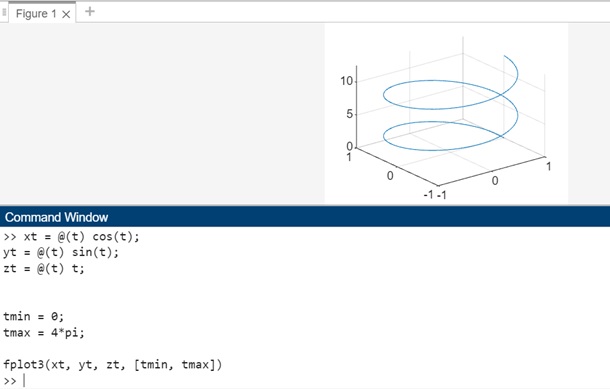
Example 2: Using fplot3(xt,yt,zt,[tmin tmax])

Let's say we want to plot a portion of the helix in 3D space given by the parametric equations −

x(t)=cos(t)

y(t)=sin(t)

z(t)=t

Over the interval 0<t<4.

The code to plot is −

xt = @(t) cos(t);
yt = @(t) sin(t);
zt = @(t) t;

tmin = 0;
tmax = 4*pi;

fplot3(xt, yt, zt, [tmin, tmax])

In this example, the fplot3(xt, yt, zt, [tmin, tmax]) function plots a portion of the helix in 3D space over the specified interval 0<t<4. The resulting plot shows the helix extending along the z-axis as t increases from 0 to 4, forming a spiral shape in 3D space.

When the code is executed in matlab command the output is −

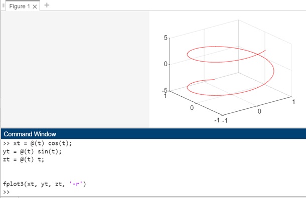
Example 3: Using fplot3(___,LineSpec)

Let's say we want to plot the parametric curve represented by the functions x(t)=cos(t), y(t)=sin(t), and z(t)=t in 3D space, and we want the curve to be displayed as a red dashed line.

The code for it is −

xt = @(t) cos(t);
yt = @(t) sin(t);
zt = @(t) t;

fplot3(xt, yt, zt, '-r')

In this example, the fplot3(xt, yt, zt, '-r') function plots the parametric curve in 3D space using the specified parametric equations and LineSpec -r (dashed red line). The resulting plot shows the curve in red color with a dashed line style.

When the code is executed the output is −

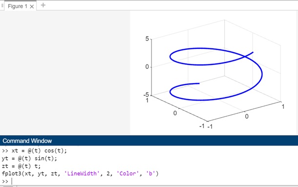
Example 4: Using fplot3(___,Name,Value)

Let's say we want to plot the parametric curve represented by the functions x(t)=cos(t), y(t)=sin(t), and z(t)=t in 3D space, and we want the curve to be displayed with a thicker line width and a blue color.

The code we have is −

xt = @(t) cos(t);
yt = @(t) sin(t);
zt = @(t) t;
fplot3(xt, yt, zt, 'LineWidth', 2, 'Color', 'b')

In this example, the fplot3(xt, yt, zt, 'LineWidth', 2, 'Color', 'b') function plots the parametric curve in 3D space using the specified parametric equations and line properties. The resulting plot shows the curve with a thicker line width of 2 points and a blue color.

When you execute the code in matlab command window the output is −

Print Page