MATLAB - Logarithmic Axes Plots

Quiz

Logarithmic axes plots in MATLAB provide a powerful tool for visualizing data that spans several orders of magnitude. Unlike linear axes, where the spacing between tick marks is constant, logarithmic axes use a logarithmic scale, allowing you to represent a wide range of values more effectively. This is particularly useful when dealing with data that exhibits exponential growth or decay, as logarithmic scales can compress large ranges into a more readable format.

What is Logarithmic Scale?

A logarithmic scale is based on the logarithm of a number. In the context of plotting, logarithmic scales transform the data by taking the logarithm of each data point. This transformation helps in displaying data that covers a large range of values, making it easier to identify trends and patterns, especially in datasets with both small and large values.

The logarithmic scale is particularly beneficial when dealing with phenomena that exhibit exponential behavior. For instance, in scientific and engineering applications, data such as signal strength, earthquake magnitude, and population growth often span several orders of magnitude, making logarithmic scales a suitable choice for representation.

Here are a few ways in which you can plot logarithmic scales.

Using loglog() Method
Using semilogx() Method

Using loglog() Method

The loglog() method helps with log scale plotting. Here is the syntax for it.

Syntax

loglog(X,Y)
loglog(X,Y,LineSpec)
loglog(X1,Y1,...,Xn,Yn)
loglog(X1,Y1,LineSpec1,...,Xn,Yn,LineSpecn)
loglog(Y)
loglog(Y,LineSpec)

The detailed explanation of the syntax is as follows −

loglog(X,Y) − The loglog function in MATLAB is designed to create plots with coordinates specified in X and Y vectors, where both the x-axis and y-axis utilize a base-10 logarithmic scale. When using loglog to visualize a single set of coordinates, ensure that X and Y are vectors of the same length.

loglog(X,Y,LineSpec) − Using loglog(X, Y, LineSpec) allows you to generate a plot with the designated line style, marker, and color specified by the LineSpec parameter.

loglog(X1,Y1,...,Xn,Yn) − the syntax loglog(X1, Y1, ..., Xn, Yn) allows you to plot multiple pairs of x- and y-coordinates on a shared set of axes.

loglog(X1,Y1,LineSpec1,...,Xn,Yn,LineSpecn) − allows you to assign distinct line styles, markers, and colors to individual x-y pairs. It provides flexibility by enabling you to specify LineSpec for certain x-y pairs while omitting it for others. For instance, using loglog(X1, Y1, 'o', X2, Y2) designates markers for the first x-y pair while leaving the second pair without specific markers.

loglog(Y) − When using loglog(Y), the function plots Y against a set of implicit x-coordinates. If Y is a vector, the x-coordinates span from 1 to the length of Y. In the case of Y being a matrix, the plot includes a distinct line for each column in Y, and the x-coordinates extend from 1 to the number of rows in Y.

loglog(Y,LineSpec) − involves plotting Y against implicit x-coordinates while concurrently defining the line style, marker, and color through the specified LineSpec.

Let us work out with examples for each of the syntax we have mentioned above.

Example 1: Using loglog(X,Y)

The code is as follows −

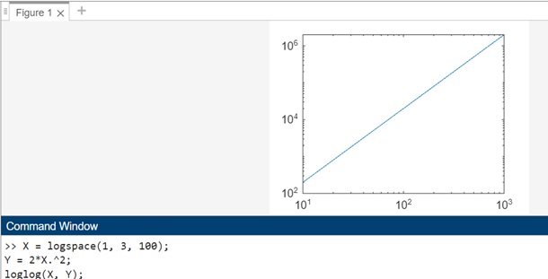
X = logspace(1, 3, 100);
Y = 2*X.^2;
loglog(X, Y);

Here the loglog function is then used to create a plot with both the x-axis and y-axis on a base-10 logarithmic scale.

When you execute the code in matlab command window the output is −

The code here is −

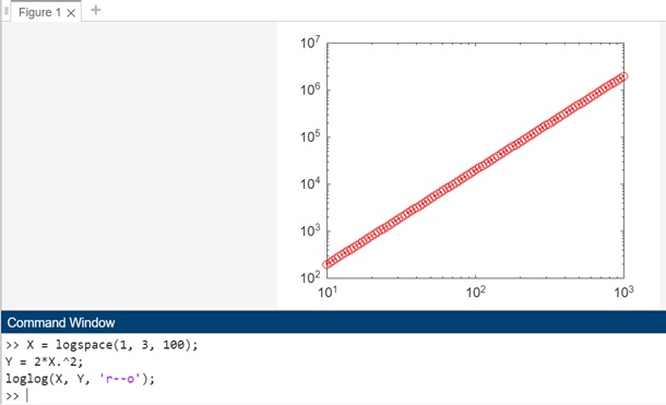
X = logspace(1, 3, 100);
Y = 2*X.^2;
loglog(X, Y, 'r--o');

In this example, the loglog(X, Y, 'r--o') syntax is used to create a plot with both the x-axis and y-axis on a base-10 logarithmic scale. The LineSpec parameter ('r--o') specifies a red dashed line with circular markers. This allows you to customize the appearance of the plot, providing a visual representation of the data with a specified line style, marker, and color.

When you execute the code in matlab command window the output is −

Example 2: Using loglog(X1,Y1,...,Xn,Yn)

The code is as follows −

X1 = logspace(1, 3, 100);
Y1 = 2*X1.^2;

X2 = logspace(1, 3, 100);
Y2 = 500./X2;

loglog(X1, Y1, 'b-', X2, Y2, 'r--');

In this example, loglog(X1, Y1, 'b-', X2, Y2, 'r--') is used to create a plot with both datasets on a base-10 logarithmic scale. The first dataset is represented by a blue solid line, and the second dataset is represented by a red dashed line. This syntax enables you to visualize and compare multiple datasets conveniently on the same set of logarithmic axes.

When you execute the code in matlab command window the output is −

Example 3: Using loglog(X1,Y1,LineSpec1,...,Xn,Yn,LineSpecn)

The code for above syntax is as shown below −

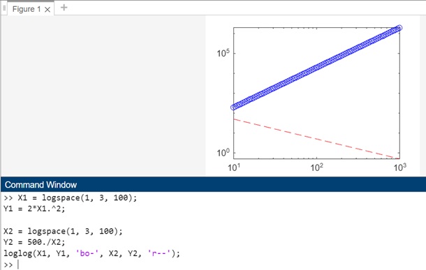
X1 = logspace(1, 3, 100);
Y1 = 2*X1.^2;

X2 = logspace(1, 3, 100);
Y2 = 500./X2;
loglog(X1, Y1, 'bo-', X2, Y2, 'r--');

In this example, loglog(X1, Y1, 'bo-', X2, Y2, 'r--') is used to create a plot with both datasets on a base-10 logarithmic scale. The first dataset is represented by blue circles connected by a solid line, and the second dataset is represented by a red dashed line. This syntax allows you to customize the appearance of each dataset individually, providing flexibility in styling for a more informative visualization.

When you execute the code in matlab command window the output is −

Example 4: Using loglog(Y)

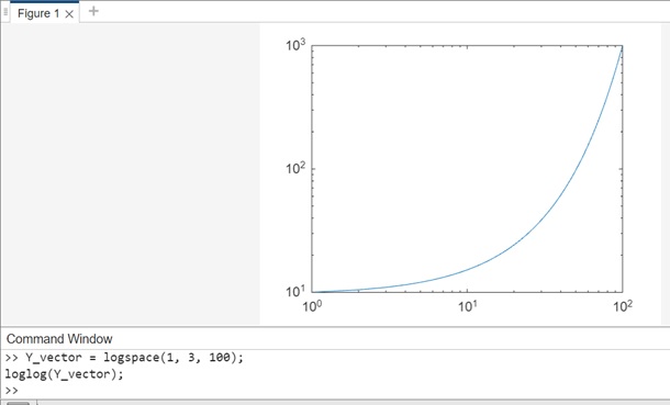
In this example, loglog(Y_vector) is used to create a loglog plot for a vector (Y_vector).

Y_vector = logspace(1, 3, 100); 
loglog(Y_vector);

When you execute the same in matlab command window the output is −

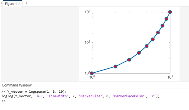
Example 5: Using loglog(Y,LineSpec)

The code for above syntax is as follows −

Y_vector = logspace(1, 3, 10);
loglog(Y_vector, 'o-', 'LineWidth', 2, 'MarkerSize', 8, 'MarkerFaceColor', 'r');

In this example, loglog(Y_vector, 'o-', 'LineWidth', 2, 'MarkerSize', 8, 'MarkerFaceColor', 'r') is used to create a loglog plot for a vector (Y_vector). The red circles are connected by a line, and the x-coordinates span from 1 to the length of the vector. Adjust the parameters as needed for your specific visualization preferences.

When you execute the same in matlab command window the output is −

Using semilogx() Method

The semilogx() function in MATLAB is used to create a plot where the x-axis is presented on a logarithmic scale, while the y-axis remains on a linear scale.

Syntax

Here is the syntax for using semilogx() method.

semilogx(X,Y)
semilogx(X,Y,LineSpec)
semilogx(X1,Y1,...,Xn,Yn)
semilogx(X1,Y1,LineSpec1,...,Xn,Yn,LineSpecn)
semilogx(Y)
semilogx(Y,LineSpec)

The detailed explanation of the syntax is as follows −

semilogx(X,Y) − it creates a plot where x- and y-coordinates are represented using a logarithmic scale with base 10 on the x-axis and a linear scale on the y-axis. When visualizing connected coordinates with line segments, ensure that X and Y are vectors of equal length.For plotting multiple sets of coordinates on a shared set of axes, it is possible to specify at least one of X or Y as a matrix.

semilogx(X,Y,LineSpec) − Using semilogx(X, Y, LineSpec) generates a plot with the defined line style, marker, and color specified by the LineSpec parameter.

semilogx(X1,Y1,...,Xn,Yn) − it facilitates the plotting of multiple sets of x- and y-coordinates on a shared set of axes. This form of syntax offers an alternative to specifying coordinates as matrices.

semilogx(X1,Y1,LineSpec1,...,Xn,Yn,LineSpecn) − it allocates distinct line styles, markers, and colors to individual x-y pairs. It provides the flexibility to specify LineSpec for certain x-y pairs while leaving it unspecified for others. For instance, in the syntax semilogx(X1, Y1, 'o', X2, Y2), markers are specified for the first x-y pair but not for the second pair.

semilogx(Y) − graphically represents Y against an inherent set of x-coordinates. In the case of a vector Y, the x-coordinates span from 1 to the length of Y. When Y is a matrix, each column contributes to a separate line on the plot, and the x-coordinates extend from 1 to the number of rows in Y.

semilogx(Y,LineSpec) − semilogx(Y, LineSpec) depicts the data in Y using implicit x-coordinates while allowing customization of the line style, marker, and color through the specified LineSpec.

Let us see a few examples for each of the syntax.

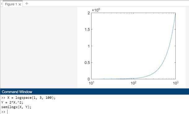
Example 1: Using semilogx(X,Y)

The code for above syntax is as follows −

X = logspace(1, 3, 100);
Y = 2*X.^2;
semilogx(X, Y);

In this example, semilogx(X, Y) creates a plot where the x-axis is represented using a logarithmic scale with a base of 10, and the y-axis is on a linear scale.

When you execute the same in matlab command window the output is −

Example 2: Using semilogx(X,Y,LineSpec)

The code for above syntax is −

X = logspace(1, 3, 100);
Y = 2*X.^2;
semilogx(X, Y, 'r--o');

In this example, semilogx(X, Y, 'r--o') generates a plot where the x-axis is on a logarithmic scale, and the y-axis is on a linear scale. The LineSpec parameter ('r--o') specifies a red dashed line with circular markers. This allows you to customize the appearance of the plot with a defined line style, marker, and color.

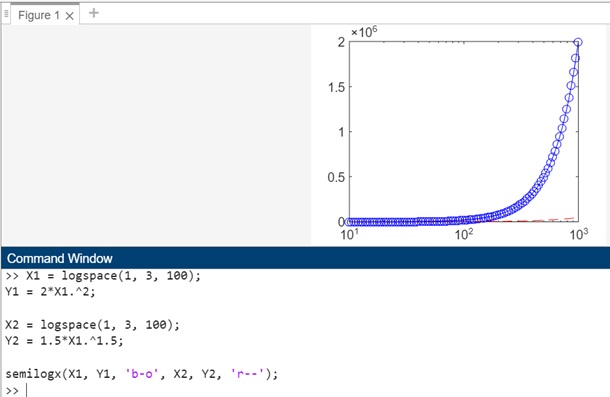
Example 3: Using semilogx(X1,Y1,...,Xn,Yn)

The code for above syntax is −

X1 = logspace(1, 3, 100);
Y1 = 2*X1.^2;

X2 = logspace(1, 3, 100);
Y2 = 1.5*X2.^1.5;

semilogx(X1, Y1, 'b-', X2, Y2, 'r--');

In this example, semilogx(X1, Y1, 'b-', X2, Y2, 'r--') is used to create a plot with both datasets on a base-10 logarithmic scale for the x-axis and a linear scale for the y-axis. The blue line represents the first dataset, and the red dashed line represents the second dataset.

When you execute the same in matlab command window the output is −

Example 4: Using semilogx(X1,Y1,LineSpec1,...,Xn,Yn,LineSpecn)

The code for above syntax is −

X1 = logspace(1, 3, 100);
Y1 = 2*X1.^2;

X2 = logspace(1, 3, 100);
Y2 = 1.5*X1.^1.5;

semilogx(X1, Y1, 'b-o', X2, Y2, 'r--');

In this example, semilogx(X1, Y1, 'b-o', X2, Y2, 'r--') is used to create a plot with both datasets on a base-10 logarithmic scale for the x-axis and a linear scale for the y-axis.

When you execute the code in matlab command window the output is −

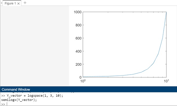
Example 5: semilogx(Y)

The code for above syntax is as follows −

Y_vector = logspace(1, 3, 10);
semilogx(Y_vector);

In this example, semilogx(Y_vector) is used to create a plot for a vector (Y_vector). The code when executed the output is as follows −

Example 6: semilogx(Y)

The syntax for above code −

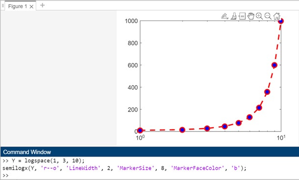
Y = logspace(1, 3, 10);
semilogx(Y, 'r--o', 'LineWidth', 2, 'MarkerSize', 8, 'MarkerFaceColor', 'b');

In this example, semilogx(Y, 'r--o', 'LineWidth', 2, 'MarkerSize', 8, 'MarkerFaceColor', 'b') is used to create a plot for a vector (Y). The red dashed line with circular markers is specified by the LineSpec parameter. Additional styling parameters such as line width, marker size, and marker face color are also customized.

When you execute the code in matlab command window the output is −

Print Page