MATLAB - Integration

---

---

Integration deals with two essentially different types of problems.

• In the first type, derivative of a function is given and we want to find the function. Therefore, we basically reverse the process of differentiation. This reverse process is known as anti-differentiation, or finding the primitive function, or finding an indefinite integral.

• The second type of problems involve adding up a very large number of very small quantities and then taking a limit as the size of the quantities approaches zero, while the number of terms tend to infinity. This process leads to the definition of the definite integral.

Definite integrals are used for finding area, volume, center of gravity, moment of inertia, work done by a force, and in numerous other applications.

Finding Indefinite Integral Using MATLAB

By definition, if the derivative of a function f(x) is f'(x), then we say that an indefinite integral of f'(x) with respect to x is f(x). For example, since the derivative (with respect to x) of x² is 2x, we can say that an indefinite integral of 2x is x².

In symbols −

f'(x²) = 2x, therefore,

∫ 2xdx = x².

Indefinite integral is not unique, because derivative of x² + c, for any value of a constant c, will also be 2x.

This is expressed in symbols as −

∫ 2xdx = x² + c.

Where, c is called an 'arbitrary constant'.

MATLAB provides an int command for calculating integral of an expression. To derive an expression for the indefinite integral of a function, we write −

int(f);

For example, from our previous example −

syms x 
int(2*x)

MATLAB executes the above statement and returns the following result −

ans =
   x^2

Example 1

In this example, let us find the integral of some commonly used expressions. Create a script file and type the following code in it −

syms x n

int(sym(x^n))
f = 'sin(n*t)'
int(sym(f))
syms a t
int(a*cos(pi*t))
int(a^x)

When you run the file, it displays the following result −

ans =
   piecewise([n == -1, log(x)], [n ~= -1, x^(n + 1)/(n + 1)])
f =
sin(n*t)
ans =
   -cos(n*t)/n
   ans =
   (a*sin(pi*t))/pi
   ans =
   a^x/log(a)

Example 2

Create a script file and type the following code in it −

syms x n
int(cos(x))
int(exp(x))
int(log(x))
int(x^-1)
int(x^5*cos(5*x))
pretty(int(x^5*cos(5*x)))

int(x^-5)
int(sec(x)^2)
pretty(int(1 - 10*x + 9 * x^2))

int((3 + 5*x -6*x^2 - 7*x^3)/2*x^2)
pretty(int((3 + 5*x -6*x^2 - 7*x^3)/2*x^2))

Note that the pretty function returns an expression in a more readable format.

When you run the file, it displays the following result −

ans =
   sin(x)
 
ans =
   exp(x)
 
ans =
   x*(log(x) - 1)
 
ans =
   log(x)
 
ans =
(24*cos(5*x))/3125 + (24*x*sin(5*x))/625 - (12*x^2*cos(5*x))/125 + (x^4*cos(5*x))/5 - (4*x^3*sin(5*x))/25 + (x^5*sin(5*x))/5
                                    2             4 
   24 cos(5 x)   24 x sin(5 x)   12 x  cos(5 x)   x  cos(5 x) 
   ----------- + ------------- - -------------- + ------------ 
      3125            625             125              5 
   
        3             5 
 
   4 x  sin(5 x)   x  sin(5 x) 
   ------------- + ----------- 
         25              5
 
ans =
-1/(4*x^4)
 
ans =
tan(x)
        2 
  x (3 x  - 5 x + 1)
 
ans = 
- (7*x^6)/12 - (3*x^5)/5 + (5*x^4)/8 + x^3/2
 
      6      5      4    3 
    7 x    3 x    5 x    x 
  - ---- - ---- + ---- + -- 
     12     5      8     2

Finding Definite Integral Using MATLAB

By definition, definite integral is basically the limit of a sum. We use definite integrals to find areas such as the area between a curve and the x-axis and the area between two curves. Definite integrals can also be used in other situations, where the quantity required can be expressed as the limit of a sum.

The int function can be used for definite integration by passing the limits over which you want to calculate the integral.

To calculate

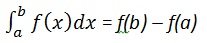
we write,

int(x, a, b)

For example, to calculate the value of we write −

int(x, 4, 9)

MATLAB executes the above statement and returns the following result −

ans =
   65/2

Following is Octave equivalent of the above calculation −

pkg load symbolic
symbols

x = sym("x");
f = x;
c = [1, 0];
integral = polyint(c);

a = polyval(integral, 9) - polyval(integral, 4);
display('Area: '), disp(double(a));

Octave executes the code and returns the following result −

Area: 

   32.500

An alternative solution can be given using quad() function provided by Octave as follows −

pkg load symbolic
symbols

f = inline("x");
[a, ierror, nfneval] = quad(f, 4, 9);

display('Area: '), disp(double(a));

Octave executes the code and returns the following result −

Area: 
   32.500

Example 1

Let us calculate the area enclosed between the x-axis, and the curve y = x³2x+5 and the ordinates x = 1 and x = 2.

The required area is given by −

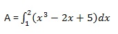
Create a script file and type the following code −

f = x^3 - 2*x +5;
a = int(f, 1, 2)
display('Area: '), disp(double(a));

When you run the file, it displays the following result −

a =
23/4
Area: 
   5.7500

Following is Octave equivalent of the above calculation −

pkg load symbolic
symbols

x = sym("x");
f = x^3 - 2*x +5;
c = [1, 0, -2, 5];
integral = polyint(c);

a = polyval(integral, 2) - polyval(integral, 1);
display('Area: '), disp(double(a));

Octave executes the code and returns the following result −

Area: 

   5.7500

An alternative solution can be given using quad() function provided by Octave as follows −

pkg load symbolic
symbols

x = sym("x");
f = inline("x^3 - 2*x +5");

[a, ierror, nfneval] = quad(f, 1, 2);
display('Area: '), disp(double(a));

Octave executes the code and returns the following result −

Area: 
   5.7500

Example 2

Find the area under the curve: f(x) = x² cos(x) for 4 x 9.

Create a script file and write the following code −

f = x^2*cos(x);
ezplot(f, [-4,9])
a = int(f, -4, 9)
disp('Area: '), disp(double(a));

When you run the file, MATLAB plots the graph −

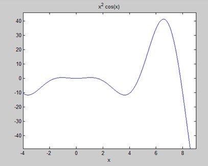
The output is given below −

a = 
8*cos(4) + 18*cos(9) + 14*sin(4) + 79*sin(9)
 
Area: 
   0.3326

Following is Octave equivalent of the above calculation −

pkg load symbolic
symbols

x = sym("x");
f = inline("x^2*cos(x)");

ezplot(f, [-4,9])
print -deps graph.eps

[a, ierror, nfneval] = quad(f, -4, 9);
display('Area: '), disp(double(a));