MATLAB - Filter Function

Quiz

The filter function in MATLAB is a powerful tool for processing one-dimensional (1-D) digital signals. It enables you to apply digital filters to your data, allowing for tasks such as noise reduction, smoothing, and feature extraction.

Syntax

The filter function, with the syntax y = filter(b, a, x), is used to apply filtering to the input data x by utilizing a rational transfer function characterized by the numerator coefficients b and the denominator coefficients a.

Depending on the input data type −

If x is a vector, the filter function will produce filtered data in the form of a vector, maintaining the same size as the original x.
When x is a matrix, filter operates along the first dimension (columns) and returns filtered data for each column of the matrix.
In the case of x being a multidimensional array, filter operates along the first dimension of the array where the size is not equal to 1.

Examples on Matlab Filter Function

Here are few examples on matlab filter function −

Example 1: Moving-Average Filter

A Moving Average filter, is a common digital signal processing technique used to smooth or reduce noise in time-series data.

Imagine you have a noisy 1-D signal, and you want to apply a simple moving average filter to smooth it. Here's how you can use the filter function for this purpose −

% Define the moving average filter coefficients
b = [1/3, 1/3, 1/3]; % Numerator coefficients
a = 1; % Denominator coefficients

% Generate a noisy signal
t = 0:0.1:10;
x = sin(t) + 0.3 * randn(size(t));

% Apply the filter
y = filter(b, a, x);

% Plot the original and filtered signals
subplot(2, 1, 1);
plot(t, x, 'b', 'LineWidth', 2);
title('Original Noisy Signal');
xlabel('Time');
ylabel('Amplitude');

subplot(2, 1, 2);
plot(t, y, 'r', 'LineWidth', 2);
title('Filtered Signal (Moving Average)');
xlabel('Time');
ylabel('Amplitude');

In this example, we define a moving average filter with coefficients b and a.

The coefficients are defined as per Moving Average filter. In this case, b represents the numerator coefficients, which are [1/3, 1/3, 1/3], indicating that each data point in the window contributes equally to the average. a represents the denominator coefficients, and for a Moving Average filter, it's typically set to 1.

The noisy signal is created by using a time vector t ranging from 0 to 10 with a step of 0.1. Then, you generate a noisy signal x by adding random noise (generated using randn) to a sine wave signal. This simulates a signal with added noise.

The filter function is used to apply the Moving Average filter (b and a) to the noisy signal x, resulting in the filtered signal y.

A figure with two subplots (two rows and one column). In the first subplot, you plot the original noisy signal x with a blue, thick line and label the axes. In the second subplot, you plot the filtered signal y with a red, thick line and label the axes.

When execute the code in matlab the output is −

Example 2: Filter Matrix Rows

We are going to filter matrix rows using a rational transfer function. A rational transfer function, describes the relationship between the input and output in control theory and signal processing.It is a fundamental concept used to model and analyze the behavior of systems that respond to inputs over time.

Let us first define the numerator and denominator coefficients for the rational transfer function.

b = 1;
a = [1 -0.2];

b = 1; − In this line, b is set to 1. This corresponds to the numerator coefficients of the filter transfer function, indicating that the filter doesn't modify the input.

a = [1 -0.2]; − A represents the denominator coefficients of the filter transfer function. The coefficients [1 -0.2] define a simple Infinite Impulse Response (IIR) filter with a single pole at 0.2. This filter will have a smoothing effect.

Let us generate random matrix x with values 2 to 15.

% Initialize the random number generator with the default seed
rng default;

% Generate a random matrix x with 2 rows and 15 columns
x = rand(2, 15)

rng default; − This command initializes the MATLAB random number generator with its default seed. Setting the random number generator to its default state ensures that you get reproducible random numbers.

x = rand(2, 15); − Here, a 2x15 matrix x is generated with random values drawn from a uniform distribution between 0 and 1. This matrix represents your input data.

Let us use the filter function on input x

y = filter(b, a, x, [], 2);

y = filter(b, a, x, [], 2); − The filter function is used to filter the input matrix x along the second dimension (columns) using the specified coefficients b and a. The empty brackets [] indicate that no initial conditions are provided. The result is stored in y, which represents the filtered data.

Let us create index vector to plot the graph

t = 0:length(x) - 1;

t = 0:length(x) - 1; − This line creates an index vector t that spans from 0 to the length of the input data minus 1.

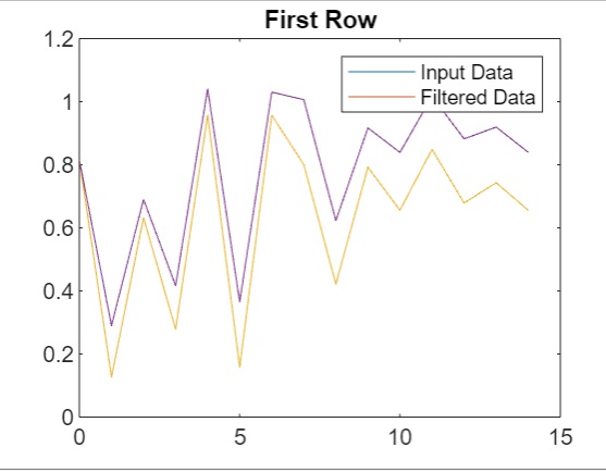
Now let us write the code for data plotting −

plot(t,x(1,:))
hold on
plot(t,y(1,:))
legend('Input Data','Filtered Data')
title('First Row')

The complete code is as follows −

rng default  %initialize random number generator
x = rand(2,15);

b = 1;
a = [1 -0.2];

y = filter(b,a,x,[],2);

t = 0:length(x)-1;  %index vector

plot(t,x(1,:))
hold on
plot(t,y(1,:))
legend('Input Data','Filtered Data')
title('First Row')

plot(t,x(1,:))
hold on
plot(t,y(1,:))
legend('Input Data','Filtered Data')
title('First Row')

The output in matlab is as follows −

Print Page