MATLAB - Linear Interpolation

Quiz

Linear interpolation is a method used to estimate values between two known data points. In this method, a straight line is drawn between the two points, and the value at any intermediate point along the line is calculated based on the known values at the endpoints. Linear interpolation is commonly used in various applications, such as signal processing, computer graphics, and data analysis, to estimate unknown values from a set of known data points.

Syntax

vq = interp1(x,v,xq)
vq = interp1(x,v,xq,method)
vq = interp1(x,v,xq,method,extrapolation)
vq = interp1(v,xq)

Here is an explanation for the syntax −

vq = interp1(x,v,xq) − Calculates new values vq by estimating points between existing data points in v. The known points are specified by x and v, where x is the sample points and v is the corresponding values. The function calculates values at positions specified by xq. If v contains multiple sets of data sampled at the same points, each column of v represents a different set of sample values.

vq = interp1(x,v,xq,method) − Allows you to choose a specific method for interpolation. The method parameter specifies how the function should estimate values between known points. The available methods include 'linear', 'nearest', 'next', 'previous', 'pchip', 'cubic', 'v5cubic', 'makima', or 'spline'. The default method is 'linear', which creates a straight line between points.

vq = interp1(x,v,xq,method,extrapolation) − Allows you to specify how to handle points that are outside the range of the known data points x. If you set extrapolation to 'extrap', the function uses the specified interpolation method to estimate values for points outside the range. Alternatively, you can specify a single value, and interp1() will return that value for all points outside the range of x.

vq = interp1(v,xq) − Calculates interpolated values assuming a default set of sample point coordinates. The default coordinates are the sequence of numbers from 1 to n, where n depends on the shape of v −

If v is a vector, the default coordinates are 1 to the length of v.
If v is an array, the default coordinates are 1 to the number of rows in v.

Examples of Linear Interpolation in MATLAB

Here are some common examples linear interpolation in matlab −

Example 1: Using vq = interp1(x,v,xq)

The code we have is as follows −

x = [1, 2, 3, 4, 5];
v = [10, 20, 15, 25, 30];
xq = 1.5:0.5:4.5;

% Perform linear interpolation
vq = interp1(x, v, xq);

% Plot the original data points
figure;
plot(x, v, 'bo-', 'LineWidth', 1.5, 'MarkerSize', 8);
hold on;

% Plot the interpolated values
plot(xq, vq, 'rx-', 'LineWidth', 1.5, 'MarkerSize', 8);

% Add labels and legend
xlabel('x');
ylabel('Value');
title('Linear Interpolation Example');
legend('Original Data', 'Interpolated Values', 'Location', 'best');
grid on;
hold off;

In the example −

We define x as the sample points [1, 2, 3, 4, 5] and v as the corresponding values [10, 20, 15, 25, 30].
xq is defined as the query points for interpolation, ranging from 1.5 to 4.5 with a step size of 0.5.
The interp1() function is used to interpolate values at the query points xq based on the known points (x, v).
The interpolated values vq are calculated and displayed. Each element of vq corresponds to the interpolated value at the respective query point in xq.
The code will plot the original data points as blue circles connected by lines ('bo-') and the interpolated values as red crosses connected by lines ('rx-').

When the code is executed the output we have is as follows −

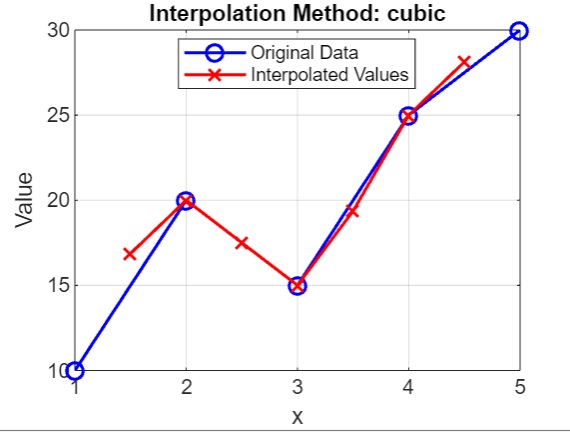
Example 2: Using vq = interp1(x,v,xq,method), with method as cubic

The code we have is −

x = [1, 2, 3, 4, 5];
v = [10, 20, 15, 25, 30];

xq = 1.5:0.5:4.5;

% Perform interpolation with different methods

method = 'cubic';
vq = interp1(x, v, xq, method);

% Plot the interpolated values

plot(x, v, 'bo-', 'LineWidth', 1.5, 'MarkerSize', 8);
hold on;
plot(xq, vq, 'rx-', 'LineWidth', 1.5, 'MarkerSize', 8);
xlabel('x');
ylabel('Value');
title(['Interpolation Method: ', method]);
legend('Original Data', 'Interpolated Values', 'Location', 'best');
grid on;
hold off;

In the example above we have −

We define x as the sample points [1, 2, 3, 4, 5] and v as the corresponding values [10, 20, 15, 25, 30].
We define query points xq for interpolation, ranging from 1.5 to 4.5 with a step size of 0.5.
We have used methods as cubic , the available options for methods are 'nearest', 'next', 'previous', 'linear', 'pchip', 'cubic', 'spline'.
We use interp1() to calculate the interpolated values vq and finally the original data points and the interpolated values for method cubic is plotted. The original data points as blue circles and the interpolated values as red crosses, with a title indicating the interpolation method used.

On execution the output we get is −

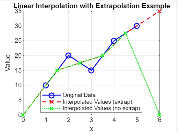
Example 3: Extrapolation using vq = interp1(x,v,xq,method,extrapolation)

The code we have is as follows −

x = [1, 2, 3, 4, 5];
v = [10, 20, 15, 25, 30];

xq = [0, 1.5, 2.5, 3.5, 4.5, 6];

% Perform linear interpolation with 'extrap' extrapolation
vq_extrap = interp1(x, v, xq, 'linear', 'extrap');

% Perform linear interpolation without extrapolation
vq_no_extrap = interp1(x, v, xq, 'linear', 0);

figure;
plot(x, v, 'bo-', 'LineWidth', 1.5, 'MarkerSize', 8);
hold on;

plot(xq, vq_extrap, 'rx--', 'LineWidth', 1.5, 'MarkerSize', 8);
plot(xq, vq_no_extrap, 'gx:', 'LineWidth', 1.5, 'MarkerSize', 8);

xlabel('x');
ylabel('Value');
title('Linear Interpolation with Extrapolation Example');
legend('Original Data', 'Interpolated Values (extrap)', 'Interpolated Values (no extrap)', 'Location', 'best');
grid on;
hold off;

In the example above we have −

We define x as the sample points [1, 2, 3, 4, 5] and v as the corresponding values [10, 20, 15, 25, 30].
We define query points xq for interpolation, including some points outside the range of x (e.g., 0 and 6).
We use interp1() to calculate the interpolated values vq_extrap with 'extrap' extrapolation and vq_no_extrap without extrapolation.
We plot the original data points as blue circles, vq_extrap as red crosses with dashed lines, and vq_no_extrap as green crosses with dotted lines.

When the code is executed the output we get is as follows −

Example 4: Default Sample Points using vq = interp1(v,xq)

The code we have is as follows −

v = [10, 20, 15, 25, 30];

xq = 1.5:0.5:5.5;

% Perform linear interpolation assuming default sample point coordinates
vq = interp1(v, xq);

% Plot the original values and the interpolated values
figure;
plot(1:length(v), v, 'bo-', 'LineWidth', 1.5, 'MarkerSize', 8);
hold on;
plot(xq, vq, 'rx-', 'LineWidth', 1.5, 'MarkerSize', 8);
xlabel('Sample Point Index');
ylabel('Value');
title('Linear Interpolation Example with Default Sample Points');
legend('Original Values', 'Interpolated Values', 'Location', 'best');
grid on;
hold off;

In the example above −

We define v as the values [10, 20, 15, 25, 30] for interpolation.
We define query points xq for interpolation, ranging from 1.5 to 5.5 with a step size of 0.5.
We use interp1() to calculate the interpolated values vq assuming default sample point coordinates.
We plot the original values as blue circles connected by lines and the interpolated values as red crosses connected by lines. The x-axis represents the index of the sample points.

On execution the output is −

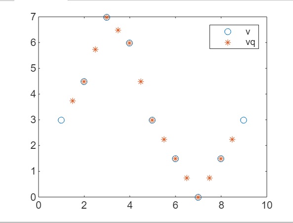
Example 5: Linear Interpolation without Points

The code we have is as follows −

v = [3, 4.5, 7, 6, 3, 1.5, 0, 1.5, 3];
xq = 1.5:0.5:8.5;
vq = interp1(1:numel(v), v, xq);
figure
plot((1:9),v,'o',xq,vq,'*');
legend('v','vq');

In the code above we have −

v = [3, 4.5, 7, 6, 3, 1.5, 0, 1.5, 3]; − Defines a vector v containing the original values for interpolation.
xq = 1.5:0.5:8.5; − Defines the query points xq for interpolation. These points range from 1.5 to 8.5 with a step size of 0.5.
vq = interp1(1:numel(v), v, xq); − Performs linear interpolation using the interp1 function. The function interpolates the values in v at the query points specified in xq. Since the sample points are not explicitly specified, the function uses the default sample point coordinates from 1 to the number of elements in v.
plot((1:9),v,'o',xq,vq,'*'); − Plots the original values v as blue circles and the interpolated values vq as red asterisks. The x-axis represents the index of the sample points.

On execution the output we get is as follows −

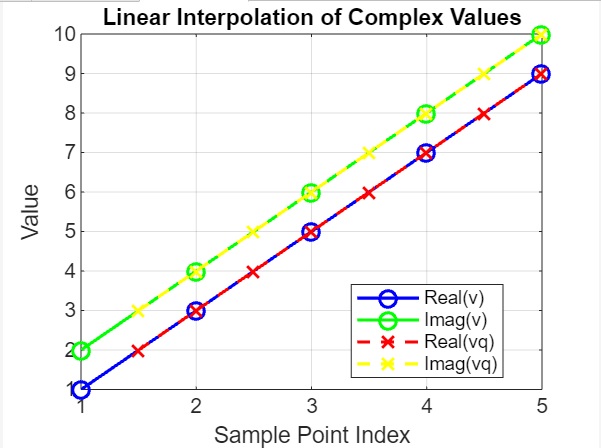
Example 6: Using Complex Numbers

The code we have is as follows −

v = [1+2i, 3+4i, 5+6i, 7+8i, 9+10i];

xq = 1.5:0.5:5.5;

% Perform linear interpolation
vq = interp1(1:numel(v), v, xq, 'linear');

% Plot the original and interpolated complex values
figure;
plot(1:numel(v), real(v), 'bo-', 1:numel(v), imag(v), 'go-', ...
   xq, real(vq), 'rx--', xq, imag(vq), 'yx--', 'LineWidth', 1.5, 'MarkerSize', 8);
xlabel('Sample Point Index');
ylabel('Value');
title('Linear Interpolation of Complex Values');
legend('Real(v)', 'Imag(v)', 'Real(vq)', 'Imag(vq)', 'Location', 'best');
grid on;

In the example above −

We define a vector v containing complex values.
We define query points xq for interpolation.
We use interp1 to perform linear interpolation on the complex values v at the query points xq.
We plot the real and imaginary parts of both the original (v) and interpolated (vq) complex values. The x-axis represents the index of the sample points.

On execution the output we have is as follows −

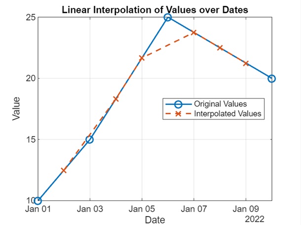
Example 7: Using Dates and Times

The code we have is as follows −

dates = datetime({'2022-01-01', '2022-01-03', '2022-01-06', '2022-01-10'}, 'InputFormat', 'yyyy-MM-dd');
values = [10, 15, 25, 20];

query_dates = datetime({'2022-01-02', '2022-01-04', '2022-01-05', '2022-01-07', '2022-01-08', '2022-01-09'}, 'InputFormat', 'yyyy-MM-dd');

% Perform linear interpolation
interp_values = interp1(dates, values, query_dates, 'linear');

% Plot the original and interpolated values
figure;
plot(dates, values, 'o-', query_dates, interp_values, 'x--', 'LineWidth', 1.5, 'MarkerSize', 8);
xlabel('Date');
ylabel('Value');
title('Linear Interpolation of Values over Dates');
legend('Original Values', 'Interpolated Values', 'Location', 'best');
grid on;

In above example −

We define a vector dates containing datetime values representing dates and a corresponding vector values containing numerical values.
We define a vector query_dates containing datetime values for which we want to interpolate values.
We use interp1 to perform linear interpolation on the original values at the dates to estimate values at the query_dates.
We plot the original values and the interpolated values over dates. The x-axis represents dates, and the y-axis represents values.

On execution the output we get is as follows −

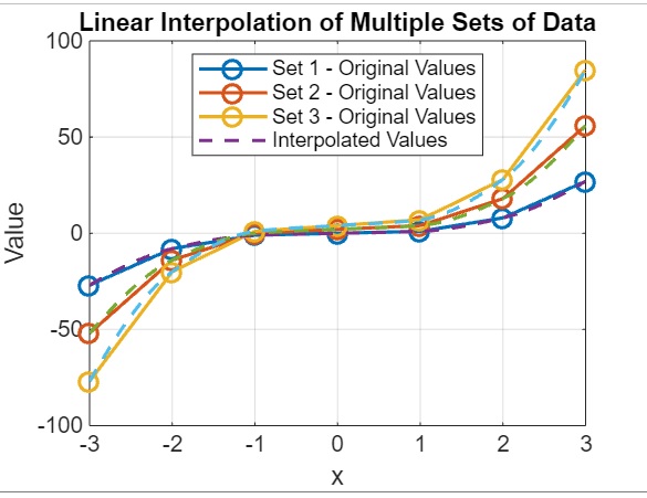
Example 8: Multiple Sets of Data

The code we have is as follows −

x = (-3:3)';
v1 = x.^3;
v2 = 2*x.^3 + 2;
v3 = 3*x.^3 + 4;

v = [v1 v2 v3];

xq = -3:0.1:3;

vq = interp1(x, v, xq, 'pchip');

% Plot the original and interpolated values for all three sets of data
figure;
plot(x, v, 'o-', xq, vq, '--', 'LineWidth', 1.5, 'MarkerSize', 8);
xlabel('x');
ylabel('Value');
title('Linear Interpolation of Multiple Sets of Data');
legend('Set 1 - Original Values', 'Set 2 - Original Values', 'Set 3 - Original Values', 'Interpolated Values', 'Location', 'best');
grid on;

In above example −

We define a vector x representing the original sample points.
We calculate three sets of original values (v1, v2, v3) using different functions of x.
We combine the original values into a single matrix v.
We define a vector xq containing query points for interpolation.
We use interp1 with the 'pchip' method to perform interpolation on the original values at the sample points to estimate values at the query points.
We plot the original values and the interpolated values for all three sets of data. The x-axis represents x, and the y-axis represents the values.

On execution the output we get is as follows −

Print Page