MATLAB - 2D Array Interpolation

Quiz

In MATLAB, 2D array interpolation is a method used to estimate values between the points of a two-dimensional grid. This is useful for creating a smoother representation of data or for increasing the resolution of an image. The interp2 function is commonly used for 2D array interpolation.

Syntax

Vq = interp2(X,Y,V,Xq,Yq)
Vq = interp2(V,Xq,Yq)
Vq = interp2(V)
Vq = interp2(V,k)
Vq = interp2(___,method)

Explanation

Vq = interp2(X,Y,V,Xq,Yq) is a function in MATLAB that helps you estimate values in between the points of a grid. When you have a set of points in a grid (X, Y) and their corresponding function values (V), interp2 can calculate the function values at other points (Xq, Yq) in the grid using linear interpolation. The interpolated values always lie on the original grid.

Vq = interp2(V,Xq,Yq) can estimate values in a grid even without specifying the exact points. It assumes a default grid that covers the entire input grid V. This default grid is useful when you want to save memory and don't need to know the exact distances between the points.

Vq = interp2(V) can estimate values in a grid even without specifying the exact points. It assumes a default grid that covers the entire input grid V. This default grid is useful when you want to save memory and don't need to know the exact distances between the points.

Vq = interp2(V,k) can estimate values in a grid by dividing the intervals between sample values. The parameter k specifies how many times to divide the intervals. This creates a finer grid with more interpolated points between the original sample values.

Vq = interp2(___,method) allows you to choose how to estimate values between points on a grid. You can use methods like 'linear', 'nearest', 'cubic', 'makima', or 'spline'. The default method is 'linear', which creates straight lines between points.

Examples for Array Interpolation

Here let us try out a few examples on array interpolation using the syntax mentioned above.

Example 1

Following is an example to calculate array interpolation using Vq = interp2(X,Y,V,Xq,Yq) −

[X, Y] = meshgrid(1:4, 1:4);
V = [5 6 7 8; 9 10 11 12; 13 14 15 16; 17 18 19 20];

[Xq, Yq] = meshgrid(1:0.5:4, 1:0.5:4);

% Perform 2D linear interpolation
Vq = interp2(X, Y, V, Xq, Yq);

% Plot the original surface
figure;
surf(X, Y, V);
title('Original Surface');
xlabel('X');
ylabel('Y');
zlabel('Value');

% Plot the interpolated surface
figure;
surf(Xq, Yq, Vq);
title('Interpolated Surface');
xlabel('Xq');
ylabel('Yq');
zlabel('Interpolated Value');

In the example above we have −

We first create a grid of sample points (X, Y) using meshgrid. Each point in this grid corresponds to a value in the matrix V.
Next, we create a finer grid of query points (Xq, Yq) by dividing the intervals between sample points by 2 in each dimension. These are the points where we want to interpolate the values.
We use the interp2 function to perform linear interpolation on the original grid (X, Y) using the query points (Xq, Yq).
We use the surf function to create a surface plot of the original data (X, Y, V). This shows the original surface represented by the matrix V.
We use the surf function again to create a surface plot of the interpolated values (Xq, Yq, Vq). This shows how the interpolation has estimated values at the query points (Xq, Yq).
By comparing the original surface with the interpolated surface, we can visually see how the interpolation has filled in the gaps between the original data points.

On code execution the output we get is as follows −

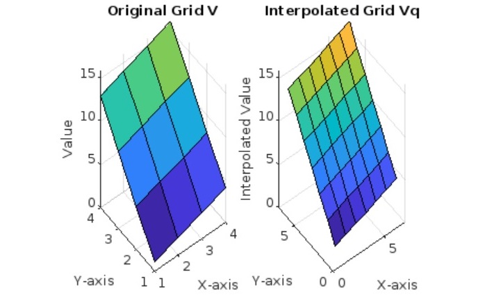
Example 2

Following is an example to calculate array interpolation using Vq = interp2(V,Xq,Yq) −

V = [1 2 3 4; 5 6 7 8; 9 10 11 12; 13 14 15 16];

[Xq, Yq] = meshgrid(1:0.5:4, 1:0.5:4);

Vq = interp2(V, Xq, Yq);

% Plot the original grid V
subplot(1, 2, 1);
surf(V);
title('Original Grid V');
xlabel('X-axis');
ylabel('Y-axis');
zlabel('Value');

% Plot the interpolated grid Vq
subplot(1, 2, 2);
surf(Vq);
title('Interpolated Grid Vq');
xlabel('Xq-axis');
ylabel('Yq-axis');
zlabel('Interpolated Value');

In the example above we have −

We start by defining a 4x4 grid of sample points represented by the matrix V.
We create a finer grid of query points (Xq, Yq) using meshgrid. These points are where we want to interpolate the values from the original grid.
We use the interp2 function to perform linear interpolation on the entire input grid V using the query points (Xq, Yq).
We plot the original grid V and the interpolated grid Vq using the surf function to visualize the surfaces. The subplotting is used to display both plots side by side for comparison.

The output on execution is as follows −

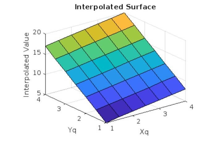
Example 3

Following is an example to calculate array interpolation using Vq = interp2(V) −

V = [1 2 3 4; 5 6 7 8; 9 10 11 12; 13 14 15 16];

Vq = interp2(V);

% Plot the original grid V
subplot(1, 2, 1);
surf(V);
title('Original Grid V');
xlabel('X-axis');
ylabel('Y-axis');
zlabel('Value');

% Plot the interpolated grid Vq
subplot(1, 2, 2);
surf(Vq);
title('Interpolated Grid Vq');
xlabel('X-axis');
ylabel('Y-axis');
zlabel('Interpolated Value');

In the example above we have −

We start by defining a 4x4 grid of sample points represented by the matrix V.
We use the interp2 function without specifying Xq and Yq, which causes it to use a default grid that covers the entire input grid V. This default grid is used to estimate values at intermediate points.
We plot the original grid V and the interpolated grid Vq using the surf function to visualize the surfaces. The subplotting is used to display both plots side by side for comparison.

On code execution the output we get is as follows −

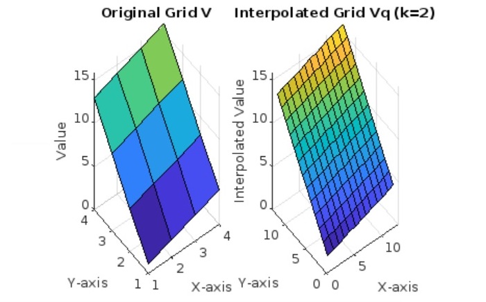
Example 4

Following is an example to calculate array interpolation using Vq = interp2(V,k) −

V = [1 2 3 4; 5 6 7 8; 9 10 11 12; 13 14 15 16];

k = 2;
Vq = interp2(V, k);

% Plot the original grid V
subplot(1, 2, 1);
surf(V);
title('Original Grid V');
xlabel('X-axis');
ylabel('Y-axis');
zlabel('Value');

% Plot the interpolated grid Vq
subplot(1, 2, 2);
surf(Vq);
title('Interpolated Grid Vq (k=2)');
xlabel('X-axis');
ylabel('Y-axis');
zlabel('Interpolated Value');

In the example above we have −

We start by defining a 4x4 grid of sample points represented by the matrix V.
We use the interp2 function with the parameter k=2, which specifies that the intervals between sample values should be divided into two parts. This creates a finer grid with more interpolated points between the original sample values.
We plot the original grid V and the interpolated grid Vq using the surf function to visualize the surfaces. The subplotting is used to display both plots side by side for comparison.

On code execution the output we get is as follows −

Example 5

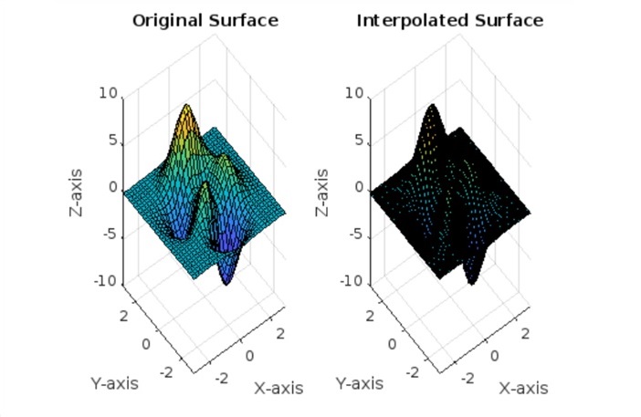
Following is an example to calculate array interpolation using Vq = interp2(___,method) −

[X, Y] = meshgrid(-3:0.2:3, -3:0.2:3);

Z = peaks(X, Y);

[Xq, Yq] = meshgrid(-3:0.05:3, -3:0.05:3);

% Perform 2D linear interpolation
Zq = interp2(X, Y, Z, Xq, Yq, 'linear');

% Plot the original and interpolated surfaces
subplot(1, 2, 1);
surf(X, Y, Z);
title('Original Surface');
xlabel('X-axis');
ylabel('Y-axis');
zlabel('Z-axis');

subplot(1, 2, 2);
surf(Xq, Yq, Zq);
title('Interpolated Surface');
xlabel('X-axis');
ylabel('Y-axis');
zlabel('Z-axis');

In the example above we have −

The meshgrid function creates a grid of points (X, Y) spanning from -3 to 3 with a step size of 0.2.
The peaks function is then used to calculate Z values based on the X and Y grid.
Another grid (Xq, Yq) is created with a finer step size of 0.05 for interpolation.
interp2 is used to perform 2D linear interpolation between the original (X, Y, Z) grid and the finer (Xq, Yq) grid, resulting in interpolated Zq values.
Both the original and interpolated surfaces are plotted using the surf function to visualize the interpolation process.

On code execution the output we get is as follows −

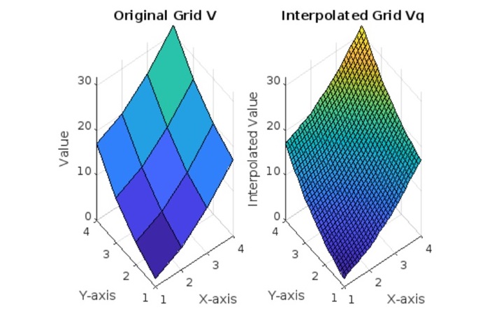
Example 6

Following is an example to calculate array interpolation using over a grid −

[X, Y] = meshgrid(1:4, 1:4);
V = X.^2 + Y.^2;

[Xq, Yq] = meshgrid(1:0.1:4, 1:0.1:4);

% Perform 2D linear interpolation
Vq = interp2(X, Y, V, Xq, Yq, 'linear');

% Plot the original and interpolated surfaces
subplot(1, 2, 1);
surf(X, Y, V);
title('Original Grid V');
xlabel('X-axis');
ylabel('Y-axis');
zlabel('Value');

subplot(1, 2, 2);
surf(Xq, Yq, Vq);
title('Interpolated Grid Vq');
xlabel('X-axis');
ylabel('Y-axis');
zlabel('Interpolated Value');

In the example above we have −

We create a grid of sample points (X, Y) using meshgrid.V is defined as a function of X and Y. In this case, V = X^2 + Y^2.
We create a finer grid (Xq, Yq) using meshgrid to define the points where we want to interpolate the values.
We use the interp2 function to interpolate the values of V at points (Xq, Yq). The 'linear' method is used for interpolation.
We plot the original grid V and the interpolated grid Vq using the surf function to visualize the surfaces. The subplotting is used to display both plots side by side for comparison.

On code execution the output we get is as follows −

Print Page