MATLAB - 3D Plots

---

---

MATLAB offers powerful tools for creating three-dimensional visualizations that allow users to represent and explore data in 3D space. 3D plots are essential for visualizing complex data, such as surfaces, volumes, and multi-dimensional datasets.

Types of 3D Plots

• Surface Plots − These visualize functions of two variables using a surface that represents the relationship between the variables.
• Mesh Plots − Mesh plots display wireframe surfaces and are useful for visualizing functions of two variables on a grid.
• Scatter Plots − In 3D, scatter plots represent individual data points in three dimensions, often with different symbols or colors to denote different properties.

Syntax

plot3(X,Y,Z)
plot3(X,Y,Z,LineSpec)
plot3(X1,Y1,Z1,...,Xn,Yn,Zn)
plot3(X1,Y1,Z1,LineSpec1,...,Xn,Yn,Zn,LineSpecn)

plot3(X,Y,Z) − This method takes care of plotting the coordinates of X,Y and Z in 3D space.

• For drawing connected coordinates through line segments, ensure X, Y, and Z are vectors of identical lengths.
• To visualize multiple coordinate sets on a single set of axes, specify at least one of X, Y, or Z as a matrix, while the rest remain vectors.

plot3(X,Y,Z,LineSpec) − This method plots a 3D with specified line style, marker and color.

plot3(X1,Y1,Z1,...,Xn,Yn,Zn) − This method helps to plot multiple sets of coordinates on the same set of axes.

plot3(X1,Y1,Z1,LineSpec1,...,Xn,Yn,Zn,LineSpecn) − The plot3 function allows assigning distinct line styles, markers, and colors to individual XYZ triplets.LineSpec can be specified for certain triplets and left out for others. For instance, using plot3(X1,Y1,Z1,'o',X2,Y2,Z2) assigns markers to the first triplet but not to the second one.

Based on the syntax discussed above let us try out a few examples to draw 3D plots.

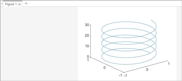
Example 1

The helix can be generated by parametric equations for x,y, and z. The general equations for a helix in cylindrical coordinates are −

Following is an example to will make use of plot3(X,Y,Z) to draw 3-D Helix −

x=r.cos(t)

y=r.sin(t)

z=h.t

Where r is the radius of the helix, t is the parameter, and h represents the pitch or vertical distance the helix travels in one complete revolution.

% Parameters
r = 1;  % Radius
h = 1;  % Pitch
t = 0:0.1:10*pi;  % Parameter range

% Parametric equations for x, y, z
x = r * cos(t);
y = r * sin(t);
z = h * t;

% Plotting the helix
plot3(x, y, z);

When you execute the same in matlab command window the output is −

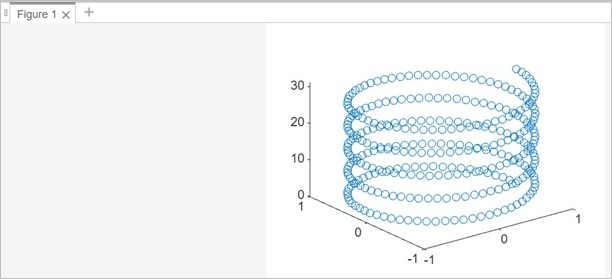
Example 2

Using the same example above let us use circular markers for the 3-D plotting

% Parameters
r = 1;  % Radius
h = 1;  % Pitch
t = 0:0.1:10*pi;  % Parameter range

% Parametric equations for x, y, z
x = r * cos(t);
y = r * sin(t);
z = h * t;

% Plotting the helix
plot3(x, y, z, 'o');

When you execute the same in matlab command window the output is −

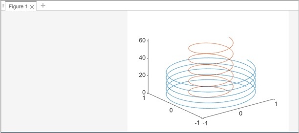
Example 3

Let us use this plot3(X1,Y1,Z1,...,Xn,Yn,Zn) to plot multiple lines for 3-D.

% Define parameters and range
t = 0:0.1:10*pi;  % Parameter range

% Line 1
r1 = 1;  % Radius of the first helix
h1 = 1;  % Pitch of the first helix
x1 = r1 * cos(t);
y1 = r1 * sin(t);
z1 = h1 * t;

% Line 2
r2 = 0.5;  % Radius of the second helix
h2 = 2;    % Pitch of the second helix
x2 = r2 * cos(t);
y2 = r2 * sin(t);
z2 = h2 * t;

% Plotting multiple lines
plot3(x1, y1, z1,x2, y2, z2);

When you execute the same in matlab the output is as follows −

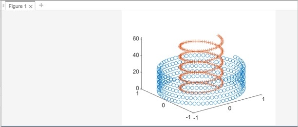
Example 4

plot3(X1,Y1,Z1,LineSpec1,...,Xn,Yn,Zn,LineSpecn) , let us specify the line style for the multiple line 3-D plotting.

% Define parameters and range
t = 0:0.1:10*pi;  % Parameter range

% Line 1
r1 = 1;  % Radius of the first helix
h1 = 1;  % Pitch of the first helix
x1 = r1 * cos(t);
y1 = r1 * sin(t);
z1 = h1 * t;

% Line 2
r2 = 0.5;  % Radius of the second helix
h2 = 2;    % Pitch of the second helix
x2 = r2 * cos(t);
y2 = r2 * sin(t);
z2 = h2 * t;

% Plotting multiple lines
plot3(x1, y1, z1,'o',x2, y2, z2,'+');

For the first line we have used circular(o) markers and the 2nd line we have used plus(+) line style.

When the code is executed the output is as follows −

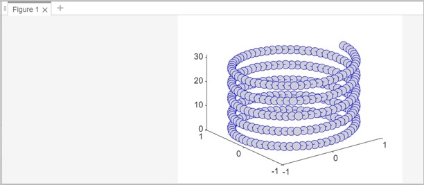
Example 5

In this example will see the customization of the marker and line styling.

% Parameters
r = 1;  % Radius
h = 1;  % Pitch
t = 0:0.1:10*pi;  % Parameter range

% Parametric equations for x, y, z
x = r * cos(t);
y = r * sin(t);
z = h * t;

% Plotting the helix
plot3(x, y, z,'-o','Color','b','MarkerSize',10,'MarkerFaceColor','#CFCFCF')

When you execute the same in matlab command window the output is −