MATLAB - Plot Mesh Surface

Quiz

Plotting mesh surfaces in MATLAB allows you to visualize functions of two variables in three-dimensional space. This is useful for understanding the behavior of functions and exploring their properties. MATLAB provides the mesh and surf functions for creating mesh and surface plots, respectively.

The mesh function in MATLAB creates a wireframe mesh plot, where the surface is represented by connecting lines. The surf function, on the other hand, creates a surface plot with colored surfaces, providing a more visually appealing representation.

Syntax

mesh(X,Y,Z)
mesh(Z)
mesh(Z,C)
mesh(ax,___)
mesh(___,Name,Value)
s = mesh(___)

Let us understand each of the syntax in detail −

mesh(X,Y,Z) − Makes a 3D surface plot with solid edge colors and no face colors. It uses matrix Z values as heights above a grid in the x-y plane defined by X and Y. The edge colors change based on the heights in Z.

mesh(Z) − Makes a mesh plot and uses the row and column numbers of the elements in Z as the x and y coordinates.

mesh(Z,C) − Tells the plot how to color the edges.

mesh(ax,___) − Plots on the axes you choose, not the current one. You need to provide the axes as the first input.

mesh(___,Name,Value) − Lets you set how the surface looks using words like 'FaceAlpha',0.5 to make it semi-transparent.

s = mesh(___) − Gives you the surface object of the chart. You can use s to change the mesh plot later.

Examples of Mesh Plotting

Let us see a few examples with the mesh Plotting.

Example 1: Using mesh(X,Y,Z)

The code we have is −

x = -2:0.1:2;
y = -2:0.1:2;
[X, Y] = meshgrid(x, y);
Z = peaks(X, Y);
mesh(X, Y, Z);

In the code above we −

First define the x and y coordinates using x = -2:0.1:2 and y = -2:0.1:2.
Then create a grid of x and y values using meshgrid to define the x-y plane.
Using a function like peaks(X, Y), we calculate the corresponding z values based on the x-y grid.
Finally, we use the mesh function to plot the 3D surface using the x, y, and z values. The surface has solid edge colors and no face colors, and the edge colors change based on the heights in Z.

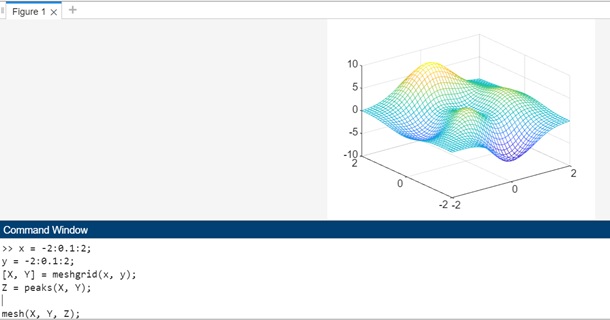
Example 2: Using the sin function to create a 3D surface plot with mesh

The code we have is as follows −

x = -2*pi:0.1:2*pi;
y = -2*pi:0.1:2*pi;
[X, Y] = meshgrid(x, y);
Z = sin(sqrt(X.^2 + Y.^2));
mesh(X, Y, Z);

In above code we have −

We define the x and y coordinates over the range of -2*pi to 2*pi.
We create a grid of x and y values using meshgrid.
The z values are calculated using the sin function applied to the square root of the sum of squares of X and Y.
Finally, we plot the 3D surface using mesh and add labels and a title to the plot.

When you execute the same in matlab command window the output is −

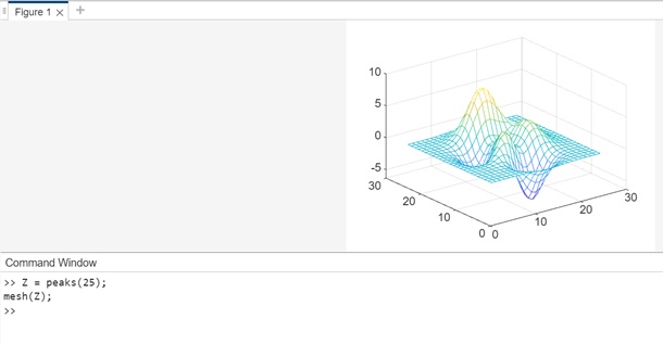
Example 3: Using mesh(Z)

The code we have is as follows −

Z = peaks(25);
mesh(Z);

In above example we have −

A matrix Z using the peaks function to generate sample data.
The mesh function is used to plot a mesh plot of Z. Since only Z is provided as input, MATLAB uses the row and column numbers of the elements in Z as the x and y coordinates, respectively.

When you execute the code in matlab command window the output is −

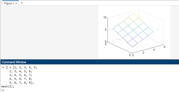
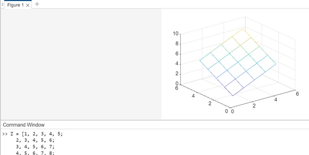
Example 4: Using matrix to plot a mesh

The code we have is −

Z = [1, 2, 3, 4, 5;
   2, 3, 4, 5, 6;
   3, 4, 5, 6, 7;
   4, 5, 6, 7, 8;
   5, 6, 7, 8, 9];
mesh(Z);

In this example, the Z matrix is a 5x5 matrix with increasing values along the rows and columns. The mesh function is used to plot a mesh plot of this custom matrix.

When you execute the matlab command window the output is −

Example 5: Using mesh(Z,C)

The code we have is −

Z = peaks(50);
C = gradient(Z);
mesh(Z, C);

In above example −

We create a matrix Z using the peaks function to generate a sample surface data.
We create a matrix C using the gradient function to define edge colors based on the values in Z.
The mesh function is used to plot a mesh plot of Z, and we specify the edge colors using the C matrix. Each element in C corresponds to an edge color for the corresponding element in Z.

When you execute the code the output is −

Example 6: Using custom matrix and custom edge color matrix to plot mesh

The code we have is −

Z = [1, 2, 3, 4, 5;
   2, 3, 4, 5, 6;
   3, 4, 5, 6, 7;
   4, 5, 6, 7, 8;
   5, 6, 7, 8, 9];
C = [0.1, 0.2, 0.3, 0.4, 0.5;
   0.2, 0.3, 0.4, 0.5, 0.6;
   0.3, 0.4, 0.5, 0.6, 0.7;
   0.4, 0.5, 0.6, 0.7, 0.8;
   0.5, 0.6, 0.7, 0.8, 0.9];

mesh(Z, C);

In above example −

We create a custom matrix Z to represent a surface.
We create another custom matrix C to define edge colors for the plot.
The mesh function is used to plot a mesh plot of Z, and we specify the edge colors using the C matrix. Each element in C corresponds to an edge color for the corresponding element in Z.

When you execute the code the output is −

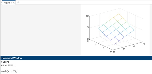
Example 7: Mesh plotting using mesh(ax,___)

The code we have is −

Z = [1, 2, 3, 4, 5;
   2, 3, 4, 5, 6;
   3, 4, 5, 6, 7;
   4, 5, 6, 7, 8;
   5, 6, 7, 8, 9];

figure;
ax = axes;

mesh(ax, Z);

In the example above we have −

We create a custom matrix Z to represent a surface.
We create a new figure and axes using the figure and axes functions.
The mesh function is used to plot a mesh plot of Z, and we specify the axes (ax) as the first input to plot on the specified axes.

When the code is executed the output is −

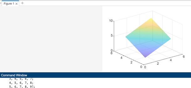
Example 8: Mesh plotting using mesh(___,Name,Value)

The code we have is −

Z = [1, 2, 3, 4, 5;
   2, 3, 4, 5, 6;
   3, 4, 5, 6, 7;
   4, 5, 6, 7, 8;
   5, 6, 7, 8, 9];


mesh(Z, 'FaceAlpha', 0.5, 'FaceColor', 'interp', 'EdgeColor', 'none');

In the code above −

We create a custom matrix Z to represent a surface.
The mesh function is used to plot a mesh plot of Z. In this example, we use additional name-value pair arguments to customize the appearance of the surface:
'FaceAlpha', 0.5 sets the transparency of the surface to 50%.
'FaceColor', 'interp' interpolates colors across the surface faces for a smooth appearance.
'EdgeColor', 'none' removes the edges of the surface for a cleaner look.

When the code is executed the output is −

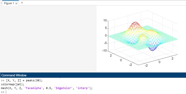
Example 9: Mesh plotting with FaceAlpha property

The code we have is as follows −

[X, Y, Z] = peaks(30);
colormap(jet);
mesh(X, Y, Z, 'FaceAlpha', 0.5, 'EdgeColor', 'interp');

In this example, the colormap(jet) command sets the colormap for the surface to the 'jet' colormap, which provides a range of colors. The 'EdgeColor', 'interp' property is used to interpolate colors for the edges of the surface.

When the code is executed the output is as follows −

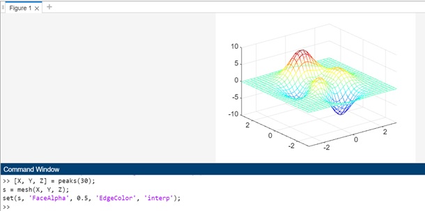
Example 10: Mesh plotting with syntax s = mesh(___)

The code we have is as follows −

[X, Y, Z] = peaks(30);
s = mesh(X, Y, Z);
set(s, 'FaceAlpha', 0.5, 'EdgeColor', 'interp');

In the example above we have −

The peaks function to generate a sample surface data with coordinates X, Y, and heights Z.
The mesh function is used to plot the mesh plot of the surface, and the output s is the handle to the surface object.
We can modify the appearance of the mesh plot later using the set function and the handle s. In this example, we modify the surface to be semi-transparent with 'FaceAlpha', 0.5 and use interpolated edge colors with 'EdgeColor', 'interp'.

The code when executed the output is −

Contour Plot Under Mesh Surface Plot

A contour plot displayed under a mesh surface plot provides a two-dimensional representation of the surface's contours projected onto the x-y plane. It offers a complementary view to the three-dimensional mesh plot by showing the contours of the surface at various levels. This allows for a more comprehensive visualization of the data, providing insights into the shape and structure of the surface. Contour plots are particularly useful for identifying regions of constant elevation or intensity on the surface and understanding its overall pattern.

Syntax

meshc(X,Y,Z)

meshc(X,Y,Z) − makes a mesh plot with contour lines underneath. The mesh plot is like a 3D surface with solid edge colors and no filled colors. It shows the heights from matrix Z on a grid formed by X and Y. The edge colors change based on the heights in Z.

Example − Contour plotting under mesh surface plot

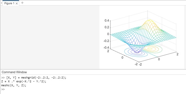
The code we have is −

[X, Y] = meshgrid(-2:.2:2, -2:.2:2);
Z = X .* exp(-X.^2 - Y.^2);
meshc(X, Y, Z);

In the example above −

We create a grid of x and y values using meshgrid and generate corresponding z values based on a function (in this case, X .* exp(-X.^2 - Y.^2)).
The meshc function is used to create a mesh plot with contour lines underneath, displaying the 3D surface along with contour lines projected onto the x-y plane beneath the surface.

When the code is executed the output we get is as follows −

Print Page