MATLAB - Transforms

---

---

MATLAB provides command for working with transforms, such as the Laplace and Fourier transforms. Transforms are used in science and engineering as a tool for simplifying analysis and look at data from another angle.

For example, the Fourier transform allows us to convert a signal represented as a function of time to a function of frequency. Laplace transform allows us to convert a differential equation to an algebraic equation.

MATLAB provides the laplace, fourier and fft commands to work with Laplace, Fourier and Fast Fourier transforms.

The Laplace Transform

The Laplace transform of a function of time f(t) is given by the following integral −

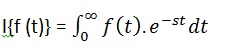
Laplace transform is also denoted as transform of f(t) to F(s). You can see this transform or integration process converts f(t), a function of the symbolic variable t, into another function F(s), with another variable s.

Laplace transform turns differential equations into algebraic ones. To compute a Laplace transform of a function f(t), write −

laplace(f(t))

Example

In this example, we will compute the Laplace transform of some commonly used functions.

Create a script file and type the following code −

syms s t a b w

laplace(a)
laplace(t^2)
laplace(t^9)
laplace(exp(-b*t))
laplace(sin(w*t))
laplace(cos(w*t))

When you run the file, it displays the following result −

ans =
   1/s^2

ans =
   2/s^3

ans =
   362880/s^10

ans =
   1/(b + s)
  
ans =
   w/(s^2 + w^2)
  
ans =
   s/(s^2 + w^2)

The Inverse Laplace Transform

MATLAB allows us to compute the inverse Laplace transform using the command ilaplace.

For example,

ilaplace(1/s^3)

MATLAB will execute the above statement and display the result −

ans =
   t^2/2

Example

Create a script file and type the following code −

syms s t a b w

ilaplace(1/s^7)
ilaplace(2/(w+s))
ilaplace(s/(s^2+4))
ilaplace(exp(-b*t))
ilaplace(w/(s^2 + w^2))
ilaplace(s/(s^2 + w^2))

When you run the file, it displays the following result −

ans =
   t^6/720

ans =
   2*exp(-t*w)

ans =
   cos(2*t)

ans =
   ilaplace(exp(-b*t), t, x)

ans =
   sin(t*w)

ans =
   cos(t*w)

The Fourier Transforms

Fourier transforms commonly transforms a mathematical function of time, f(t), into a new function, sometimes denoted by or F, whose argument is frequency with units of cycles/s (hertz) or radians per second. The new function is then known as the Fourier transform and/or the frequency spectrum of the function f.

Example

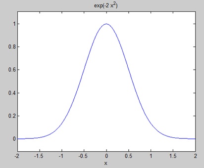
Create a script file and type the following code in it −

syms x 
f = exp(-2*x^2);     %our function
ezplot(f,[-2,2])     % plot of our function
FT = fourier(f)      % Fourier transform

When you run the file, MATLAB plots the following graph −

The following result is displayed −

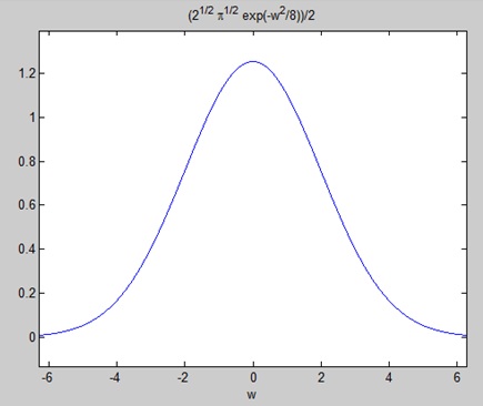
FT =
   (2^(1/2)*pi^(1/2)*exp(-w^2/8))/2

Plotting the Fourier transform as −

ezplot(FT)

Gives the following graph −

Inverse Fourier Transforms

MATLAB provides the ifourier command for computing the inverse Fourier transform of a function. For example,

f = ifourier(-2*exp(-abs(w)))

MATLAB will execute the above statement and display the result −

f =
   -2/(pi*(x^2 + 1))