- MATLAB - Home
- MATLAB - Overview
- MATLAB - Features
- MATLAB - Environment Setup
- MATLAB - Editors
- MATLAB - Online
- MATLAB - Workspace
- MATLAB - Syntax
- MATLAB - Variables
- MATLAB - Commands
- MATLAB - Data Types
- MATLAB - Operators
- MATLAB - Dates and Time
- MATLAB - Numbers
- MATLAB - Random Numbers
- MATLAB - Strings and Characters
- MATLAB - Text Formatting
- MATLAB - Timetables
- MATLAB - M-Files
- MATLAB - Colon Notation
- MATLAB - Data Import
- MATLAB - Data Output
- MATLAB - Normalize Data
- MATLAB - Predefined Variables
- MATLAB - Decision Making
- MATLAB - Decisions
- MATLAB - If End Statement
- MATLAB - If Else Statement
- MATLAB - If…Elseif Else Statement
- MATLAB - Nest If Statememt
- MATLAB - Switch Statement
- MATLAB - Nested Switch
- MATLAB - Loops
- MATLAB - Loops
- MATLAB - For Loop
- MATLAB - While Loop
- MATLAB - Nested Loops
- MATLAB - Break Statement
- MATLAB - Continue Statement
- MATLAB - End Statement
- MATLAB - Arrays
- MATLAB - Arrays
- MATLAB - Vectors
- MATLAB - Transpose Operator
- MATLAB - Array Indexing
- MATLAB - Multi-Dimensional Array
- MATLAB - Compatible Arrays
- MATLAB - Categorical Arrays
- MATLAB - Cell Arrays
- MATLAB - Matrix
- MATLAB - Sparse Matrix
- MATLAB - Tables
- MATLAB - Structures
- MATLAB - Array Multiplication
- MATLAB - Array Division
- MATLAB - Array Functions
- MATLAB - Functions
- MATLAB - Functions
- MATLAB - Function Arguments
- MATLAB - Anonymous Functions
- MATLAB - Nested Functions
- MATLAB - Return Statement
- MATLAB - Void Function
- MATLAB - Local Functions
- MATLAB - Global Variables
- MATLAB - Function Handles
- MATLAB - Filter Function
- MATLAB - Factorial
- MATLAB - Private Functions
- MATLAB - Sub-functions
- MATLAB - Recursive Functions
- MATLAB - Function Precedence Order
- MATLAB - Map Function
- MATLAB - Mean Function
- MATLAB - End Function
- MATLAB - Error Handling
- MATLAB - Error Handling
- MATLAB - Try...Catch statement
- MATLAB - Debugging
- MATLAB - Plotting
- MATLAB - Plotting
- MATLAB - Plot Arrays
- MATLAB - Plot Vectors
- MATLAB - Bar Graph
- MATLAB - Histograms
- MATLAB - Graphics
- MATLAB - 2D Line Plot
- MATLAB - 3D Plots
- MATLAB - Formatting a Plot
- MATLAB - Logarithmic Axes Plots
- MATLAB - Plotting Error Bars
- MATLAB - Plot a 3D Contour
- MATLAB - Polar Plots
- MATLAB - Scatter Plots
- MATLAB - Plot Expression or Function
- MATLAB - Draw Rectangle
- MATLAB - Plot Spectrogram
- MATLAB - Plot Mesh Surface
- MATLAB - Plot Sine Wave
- MATLAB - Interpolation
- MATLAB - Interpolation
- MATLAB - Linear Interpolation
- MATLAB - 2D Array Interpolation
- MATLAB - 3D Array Interpolation
- MATLAB - Polynomials
- MATLAB - Polynomials
- MATLAB - Polynomial Addition
- MATLAB - Polynomial Multiplication
- MATLAB - Polynomial Division
- MATLAB - Derivatives of Polynomials
- MATLAB - Transformation
- MATLAB - Transforms
- MATLAB - Laplace Transform
- MATLAB - Laplacian Filter
- MATLAB - Laplacian of Gaussian Filter
- MATLAB - Inverse Fourier transform
- MATLAB - Fourier Transform
- MATLAB - Fast Fourier Transform
- MATLAB - 2-D Inverse Cosine Transform
- MATLAB - Add Legend to Axes
- MATLAB - Object Oriented
- MATLAB - Object Oriented Programming
- MATLAB - Classes and Object
- MATLAB - Functions Overloading
- MATLAB - Operator Overloading
- MATLAB - User-Defined Classes
- MATLAB - Copy Objects
- MATLAB - Algebra
- MATLAB - Linear Algebra
- MATLAB - Gauss Elimination
- MATLAB - Gauss-Jordan Elimination
- MATLAB - Reduced Row Echelon Form
- MATLAB - Eigenvalues and Eigenvectors
- MATLAB - Integration
- MATLAB - Integration
- MATLAB - Double Integral
- MATLAB - Trapezoidal Rule
- MATLAB - Simpson's Rule
- MATLAB - Miscellenous
- MATLAB - Calculus
- MATLAB - Differential
- MATLAB - Inverse of Matrix
- MATLAB - GNU Octave
- MATLAB - Simulink
MATLAB - Plotting
To plot the graph of a function, you need to take the following steps −
Define x, by specifying the range of values for the variable x, for which the function is to be plotted
Define the function, y = f(x)
Call the plot command, as plot(x, y)
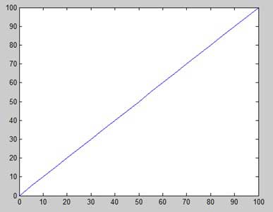
Following example would demonstrate the concept. Let us plot the simple function y = x for the range of values for x from 0 to 100, with an increment of 5.
Create a script file and type the following code −
x = [0:5:100];
y = x;
plot(x, y)
When you run the file, MATLAB displays the following plot −
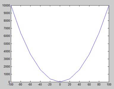
Let us take one more example to plot the function y = x2. In this example, we will draw two graphs with the same function, but in second time, we will reduce the value of increment. Please note that as we decrease the increment, the graph becomes smoother.
Create a script file and type the following code −
x = [1 2 3 4 5 6 7 8 9 10];
x = [-100:20:100];
y = x.^2;
plot(x, y)
When you run the file, MATLAB displays the following plot −
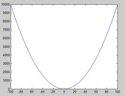
Change the code file a little, reduce the increment to 5 −
x = [-100:5:100];
y = x.^2;
plot(x, y)
MATLAB draws a smoother graph −
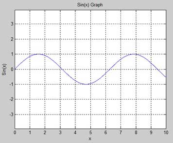
Adding Title, Labels, Grid Lines and Scaling on the Graph
MATLAB allows you to add title, labels along the x-axis and y-axis, grid lines and also to adjust the axes to spruce up the graph.
The xlabel and ylabel commands generate labels along x-axis and y-axis.
The title command allows you to put a title on the graph.
The grid on command allows you to put the grid lines on the graph.
The axis equal command allows generating the plot with the same scale factors and the spaces on both axes.
The axis square command generates a square plot.
Example
Create a script file and type the following code −
x = [0:0.01:10];
y = sin(x);
plot(x, y), xlabel('x'), ylabel('Sin(x)'), title('Sin(x) Graph'),
grid on, axis equal
MATLAB generates the following graph −
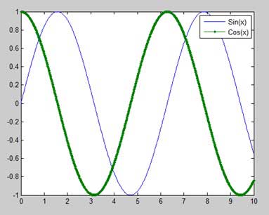
Drawing Multiple Functions on the Same Graph
You can draw multiple graphs on the same plot. The following example demonstrates the concept −
Example
Create a script file and type the following code −
x = [0 : 0.01: 10];
y = sin(x);
g = cos(x);
plot(x, y, x, g, '.-'), legend('Sin(x)', 'Cos(x)')
MATLAB generates the following graph −
Setting Colors on Graph
MATLAB provides eight basic color options for drawing graphs. The following table shows the colors and their codes −
| Code | Color |
|---|---|
| w | White |
| k | Black |
| b | Blue |
| r | Red |
| c | Cyan |
| g | Green |
| m | Magenta |
| y | Yellow |
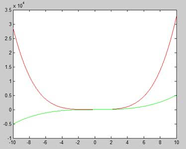
Example
Let us draw the graph of two polynomials
f(x) = 3x4 + 2x3+ 7x2 + 2x + 9 and
g(x) = 5x3 + 9x + 2
Create a script file and type the following code −
x = [-10 : 0.01: 10];
y = 3*x.^4 + 2 * x.^3 + 7 * x.^2 + 2 * x + 9;
g = 5 * x.^3 + 9 * x + 2;
plot(x, y, 'r', x, g, 'g')
When you run the file, MATLAB generates the following graph −
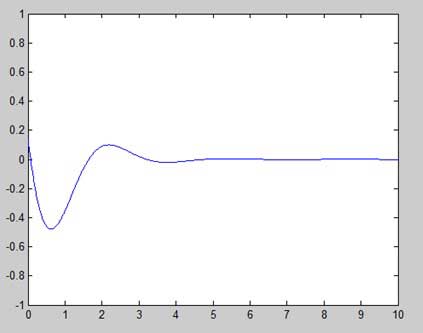
Setting Axis Scales
The axis command allows you to set the axis scales. You can provide minimum and maximum values for x and y axes using the axis command in the following way −
axis ( [xmin xmax ymin ymax] )
The following example shows this −
Example
Create a script file and type the following code −
x = [0 : 0.01: 10];
y = exp(-x).* sin(2*x + 3);
plot(x, y), axis([0 10 -1 1])
When you run the file, MATLAB generates the following graph −
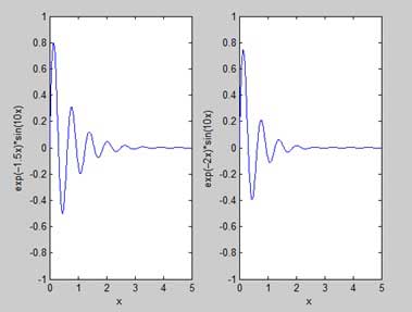
Generating Sub-Plots
When you create an array of plots in the same figure, each of these plots is called a subplot. The subplot command is used for creating subplots.
Syntax for the command is −
subplot(m, n, p)
where, m and n are the number of rows and columns of the plot array and p specifies where to put a particular plot.
Each plot created with the subplot command can have its own characteristics. Following example demonstrates the concept −
Example
Let us generate two plots −
y = e1.5xsin(10x)
y = e2xsin(10x)
Create a script file and type the following code −
x = [0:0.01:5];
y = exp(-1.5*x).*sin(10*x);
subplot(1,2,1)
plot(x,y), xlabel('x'),ylabel('exp(1.5x)*sin(10x)'),axis([0 5 -1 1])
y = exp(-2*x).*sin(10*x);
subplot(1,2,2)
plot(x,y),xlabel('x'),ylabel('exp(2x)*sin(10x)'),axis([0 5 -1 1])
When you run the file, MATLAB generates the following graph −