- OS - Home
- OS - Overview
- OS - History
- OS - Evolution
- OS - Functions
- OS - Components
- OS - Structure
- OS - Architecture
- OS - Services
- OS - Properties
- Process Management
- Processes in Operating System
- States of a Process
- Process Schedulers
- Process Control Block
- Operations on Processes
- Process Suspension and Process Switching
- Process States and the Machine Cycle
- Inter Process Communication (IPC)
- Remote Procedure Call (RPC)
- Context Switching
- Threads
- Types of Threading
- Multi-threading
- System Calls
- Scheduling Algorithms
- Process Scheduling
- Types of Scheduling
- Scheduling Algorithms Overview
- FCFS Scheduling Algorithm
- SJF Scheduling Algorithm
- Round Robin Scheduling Algorithm
- HRRN Scheduling Algorithm
- Priority Scheduling Algorithm
- Multilevel Queue Scheduling
- Lottery Scheduling Algorithm
- Starvation and Aging
- Turn Around Time & Waiting Time
- Burst Time in SJF Scheduling
- Process Synchronization
- Process Synchronization
- Solutions For Process Synchronization
- Hardware-Based Solution
- Software-Based Solution
- Critical Section Problem
- Critical Section Synchronization
- Mutual Exclusion Synchronization
- Mutual Exclusion Using Interrupt Disabling
- Peterson's Algorithm
- Dekker's Algorithm
- Bakery Algorithm
- Semaphores
- Binary Semaphores
- Counting Semaphores
- Mutex
- Turn Variable
- Bounded Buffer Problem
- Reader Writer Locks
- Test and Set Lock
- Monitors
- Sleep and Wake
- Race Condition
- Classical Synchronization Problems
- Dining Philosophers Problem
- Producer Consumer Problem
- Sleeping Barber Problem
- Reader Writer Problem
- OS Deadlock
- Introduction to Deadlock
- Conditions for Deadlock
- Deadlock Handling
- Deadlock Prevention
- Deadlock Avoidance (Banker's Algorithm)
- Deadlock Detection and Recovery
- Deadlock Ignorance
- Resource Allocation Graph
- Livelock
- Memory Management
- Memory Management
- Logical and Physical Address
- Contiguous Memory Allocation
- Non-Contiguous Memory Allocation
- First Fit Algorithm
- Next Fit Algorithm
- Best Fit Algorithm
- Worst Fit Algorithm
- Buffering
- Fragmentation
- Compaction
- Virtual Memory
- Segmentation
- Paged Segmentation & Segmented Paging
- Buddy System
- Slab Allocation
- Overlays
- Free Space Management
- Locality of Reference
- Paging and Page Replacement
- Paging
- Demand Paging
- Page Table
- Page Replacement Algorithms
- Second Chance Page Replacement
- Optimal Page Replacement Algorithm
- Belady's Anomaly
- Thrashing
- Storage and File Management
- File Systems
- File Attributes
- Structures of Directory
- Linked Index Allocation
- Indexed Allocation
- Disk Scheduling Algorithms
- FCFS Disk Scheduling
- SSTF Disk Scheduling
- SCAN Disk Scheduling
- LOOK Disk Scheduling
- I/O Systems
- I/O Hardware
- I/O Software
- I/O Programmed
- I/O Interrupt-Initiated
- Direct Memory Access
- OS Types
- OS - Types
- OS - Batch Processing
- OS - Multiprogramming
- OS - Multitasking
- OS - Multiprocessing
- OS - Distributed
- OS - Real-Time
- OS - Single User
- OS - Monolithic
- OS - Embedded
- Popular Operating Systems
- OS - Hybrid
- OS - Zephyr
- OS - Nix
- OS - Linux
- OS - Blackberry
- OS - Garuda
- OS - Tails
- OS - Clustered
- OS - Haiku
- OS - AIX
- OS - Solus
- OS - Tizen
- OS - Bharat
- OS - Fire
- OS - Bliss
- OS - VxWorks
- Miscellaneous Topics
- OS - Security
- OS Questions Answers
- OS - Questions Answers
- OS Useful Resources
- OS - Quick Guide
- OS - Useful Resources
- OS - Discussion
Shortest Job First (SJF) Scheduling
A CPU scheduling strategy is a procedure that selects one process in the waiting state and assigns it to the CPU so that it can be executed. There are a number of scheduling algorithms. In this section, we will learn about Shortest Job First or SJF scheduling algorithm.
SJF (SHORTEST JOB FIRST) Scheduling
In the Shortest Job First scheduling algorithm, the processes are scheduled in ascending order of their CPU burst times, i.e. the CPU is allocated to the process with the shortest execution time.
Variants of SJF Scheduling
There are two variants of SJF scheduling −
SJF non-preemptive scheduling
In the non-preemptive version, once a process is assigned to the CPU, it runs into completion. Here, the short term scheduler is invoked when a process completes its execution or when a new process(es) arrives in an empty ready queue.
SJF preemptive scheduling
This is the preemptive version of SJF scheduling and is also referred as Shortest Remaining Time First (SRTF) scheduling algorithm. Here, if a short process enters the ready queue while a longer process is executing, process switch occurs by which the executing process is swapped out to the ready queue while the newly arrived shorter process starts to execute. Thus the short term scheduler is invoked either when a new process arrives in the system or an existing process completes its execution.
Features of SJF Algorithm
- SJF allocates CPU to the process with shortest execution time.
- In cases where two or more processes have the same burst time, arbitration is done among these processes on first come first serve basis.
- There are both preemptive and non-premptive versions.
- It minimises the average waiting time of the processes.
- It may cause starvation of long processes if short processes continue to come in the system.
We can understand the workings of the two versions of this scheduling strategy through the aid of the following examples.
Examples of Non-Preemptive SJF Algorithm
Example 1
Suppose that we have a set of four processes that have arrived at the same time in the order P1, P2, P3 and P4. The burst time in milliseconds of each process is given by the following table −
| Process | CPU Burst Time in ms |
|---|---|
| P1 | 6 |
| P2 | 10 |
| P3 | 4 |
| P4 | 6 |
Let us draw the GANTT chart and find the average turnaround time and average waiting time using non-preemptive SJF algorithm.
GANTT Chart for the set of processes using SJF
Process P3 has the shortest burst time and so it executes first. Then we find that P1 and P4 have equal burst time of 6ms. Since P1 arrived before, CPU is allocated to P1 and then to P4. Finally P2 executes. Thus the order of execution is P3, P1, P4, P2 and is given by the following GANTT chart −

Let us compute the average turnaround time and average waiting time from the above chart.
Average Turnaround Time
=Sum of Turnaround Time of each Process / Number of Processes
= (TATP1 + TATP2 + TATP3 + TATP4) / 4
= (10 + 26 + 4 + 16) / 4 = 14 ms
Average Waiting Time
= Sum of Waiting Time of Each Process / Number of processes
= (WTP1 + WTP2 + WTP3 + WTP4) / 4
= (4 + 16 + 0 + 10) / 4 = 7.5 ms
Example 2
In the previous example, we had assumed that all the processes had arrived at the same time, a situation which is practically impossible. Here, we consider circumstance when the processes arrive at different times. Suppose we have set of four processes whose arrival times and CPU burst times are as follows −
| Process | Arrival Time | CPU Burst Time |
|---|---|---|
| P1 | 0 | 6 |
| P2 | 4 | 10 |
| P3 | 4 | 4 |
| P4 | 8 | 3 |
Let us draw the GANTT chart and find the average turnaround time and average waiting time using non-preemptive SJF algorithm.
GANTT Chart
While drawing the GANTT chart, we will consider which processes have arrived in the system when the scheduler is invoked. At time 0ms, only P1 is there and so it is assigned to CPU. P1 completes execution at 6ms and at that time P2 and P3 have arrived, but not P4. P3 is assigned to CPU since it has the shortest burst time among current processes. P3 completes execution at time 10ms. By that time P4 has arrived and so SJF algorithm is run on the processes P2 and P4. Hence, we find that the order of execution is P1, P3, P4, P2 as shown in the following GANTT chart −
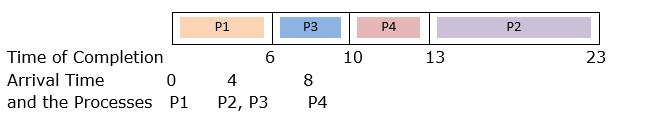
Let us calculate the turnaround time of each process and hence the average.
Turnaround Time of a process = Completion Time Arrival Time
TATP1 = CTP1 - ATP1 = 6 - 0 = 6 ms
TATP2 = CTP2 - ATP2 = 23 - 4 = 19 ms
TATP3 = CTP3 - ATP3 = 10 - 4 = 6 ms
TATP4 = CTP4 - ATP4 = 13 - 8 = 5 ms
Average Turnaround Time
=Sum of Turnaround Time of each Process/ Number of Processes
= (6 + 19+ 6 + 5) / 4 = 9 ms
The waiting time is given by the time that each process waits in the ready queue. For a non-preemptive scheduling algorithm, waiting time of each process can be simply calculated as −
Waiting Time of any process = Time of admission to CPU Arrival Time
WTP1 = 0 - 0 = 0 ms
WTP2 = 13 - 4 = 9 ms
WTP3 = 6 - 4 = 2 ms
WTP4 = 10 - 8 = 2 ms
Average Waiting Time
= Sum of Waiting Time of Each Process/ Number of processes
= (WTP1 + WTP2 + WTP3 + WTP4) / 4
= (0 + 9 + 2 + 2) / 4 = 3.25 ms
Example of Preemptive SJF (SRTF) algorithm
Let us now perform preemptive SJF (SRTN) scheduling on the following processes, draw GANTT chart and find the average turnaround time and average waiting time.
| Process | Arrival Time | CPU Burst Time |
|---|---|---|
| P1 | 0 | 8 |
| P2 | 4 | 10 |
| P3 | 4 | 3 |
| P4 | 10 | 4 |
GANTT Chart
Since this is a preemptive scheduling algorithm, the scheduler is invoked when a process arrives and when it completes execution. The scheduler computes the remaining time of completion for each of the processes in the system and selects the process having shortest remaining time left for execution.
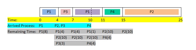
Initially, only P1 arrives and so it is assigned to CPU. At time 4ms, P2 and P3 arrive. The scheduler computes the remaining time of the processes P1, P2 and P3 as 4ms, 10ms and 3ms. Since, P3 has shortest time, P1 is pre-empted by P3. P3 completes execution at 7ms and the scheduler is invoked. Among the processes in the system, P1 has shortest time and so it executes. At time 10ms, P4 arrives and the scheduler again computes the remaining times left for each process. Since the remaining time of P1 is least, no process switch occurs and P1 continues to execute. In the similar fashion, the rest of the processes complete execution.
From the GANTT chart, we compute the average turnaround time and the average waiting time.
Average Turnaround Time
=Sum of Turnaround Time of each Process/ Number of Processes
= (TATP1 + TATP2 + TATP3 + TATP4) / 4
= ((11 - 0) + (25 - 4) + (7 - 4) + (15 - 10)) / 4 = 10 ms
Average Waiting Time
= Sum of Waiting Time of Each Process/ Number of processes
= (WTP1 + WTP2 + WTP3 + WTP4) / 4
= (3 + 11 + 0 + 1) / 4 = 3.75 ms
Advantages of SJF Algorithm
- In both preemptive and non-preemptive methods, the average waiting time is reduced substantially in SJF when compared to FCFS scheduling.
- SJF optimizes turnaround time to a considerable degree.
- If execution time of each process is estimated precisely, it promises maximum throughput.
Disadvantages of SJF Algorithm
- In situations where there is an incoming stream of processes with short burst times, longer processes in the system may be waiting in the ready queue indefinitely leading to starvation.
- In preemptive SJF, i.e. SRTF, if all processes arrive at different times and at frequent intervals, the scheduler may be always working and consequently the processor may be more engaged in process switching than actual execution of the processes.
- Correct estimation of the burst time a process is a complicated process. Since the effectiveness of the algorithm is entirely based upon the burst times, an erroneous calculation may cause inefficient scheduling.
Conclusion
Shortest Job First scheduling can be termed as the optimal scheduling algorithm due to its theoretical best results. However, the implementation is much more complex and the execution is more unpredictable than First Come First Serve or Round Robin scheduling.
