Predicting Burst Time in SJF Scheduling

---

---

In many scheduling strategies, the efficiency of the scheduler depends on the correct prediction of the burst times of the CPU processes.

Let us consider the example of Shortest Job First Scheduling (SJF) algorithm, which is the most optimal strategy with highest throughput and lowest waiting time. SJF allocates the CPU in increasing order of burst size of the processes. We observe that it is assumed that the burst sizes of the processes are available before execution.

However, no process can declare its CPU burst time beforehand as it is a dynamically changing parameter that is vastly dependent on the hardware of the computer. In absence of the availability of correct burst times, the scheduling strategy fails. This situation occurs in Highest Response Ratio Next (HRRN) and Shortest Remaining Time Next (SRTN) algorithms too.

In order that these scheduling strategies can be deployed for CPU process scheduling, a solution is to predict the burst times of the CPU processes. In this topic, we will discuss the various techniques for prediction of burst times.

Techniques of Predicting Burst Times of Processes

Burst time of processes can be found using traditional techniques or by machine learning approaches. In the traditional techniques, predictions are done based upon the burst time of the already completed processes, using either static or dynamic algorithms. The following diagram depicts the different methods −

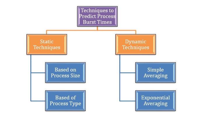
Static Techniques

These techniques perform calculation based some heuristic strategies based upon the completed processes. However, these strategies are not much accurate and consequently less reliable.

The two conventional static technique heuristics for predicting CPU burst times are based upon process size and process type, as elaborated below −

Based on Process Size

The parameter of heuristic considered in this case is the process size. The heuristic is: Burst times of processes of similar sizes are similar. So, when a process enters a system, the total memory space allotted to the process is considered. Burst times of past processes of similar size are considered. From this the burst time of the new process is predicted.

For example, consider that a process of size 250KB has arrived in the system. History data has five processes P1 to P5, with following parameters −

• P1 had size 100 KB and took 4 milliseconds for execution
• P2 had size 375 KB and took 10 milliseconds for execution
• P3 had size 170 KB and took 5 milliseconds for execution
• P4 had size 245 KB and took 7 milliseconds for execution
• P5 had size 500 KB and took 15 milliseconds for execution

It can be observed that the size of the new process is nearest to P4. And so, as per this process size heuristics, predicted burst time is 7 milliseconds.

Based on Process Type

Here, the heuristic is: Burst times of processes of similar types are similar. Processes may be system processes, user processes, real time processes, interactive processes and so on. When a new process enters the system, the type of process is ascertained and the its burst time is predicted accordingly.

For example, consider that a system has the following approximate burst times according to process types −

• Burst time of kernel processes: 4 milliseconds
• Burst time of foreground processes: 14 milliseconds
• Burst time of interactive processes: 8 milliseconds
• Burst time of background processes: 20 milliseconds

If a kernel process arrives in this system, its burst time will be predicted as 4 milliseconds as per process type heuristics.

Dynamic Techniques

Dynamic techniques consider the history of processes as a time series and predict the burst time of the next process as a function of the past processes. The two traditional dynamic methods uses simple averaging and exponential averaging, explained as follows −

Simple Average

In this method, the burst time of the next process is the simple average of the burst times of all processes in the system.

Mathematically, considering that there are n processes in the system, P₁, P₂,P₃, P_n , having burst times t₁,t₂,t₃, t_n, the burst time of the next process in the queue is given by −

$$\mathrm{t_{n+1} \: = \: \frac{1}{n}\displaystyle\sum\limits_{i=1}^n t_{i}}$$

For example, consider that there were previously 5 processes in the system with burst times 4, 6, 7, 5 and 3 milliseconds. The burst time of the next process will be (4 + 6 + 7 + 5 + 3) / 5 = 5ms.

Exponential Average

This is an improvement over simple averaging as it gives preferential weightage to recent history and past history. Here, a smoothing factor, α (0 α 1) is defined to give the relative weightage. The predicted burst time, τ_(n+1) is defined as −

$$\mathrm{\tau_{n+1} \: = \: \alpha t_{n} \: + \: (1 - \alpha)\tau_{n}}$$

where, t_n is the actual burst time of P_n and τ_n was the previous predicted burst time. We can expand this formula by substituting the subsequent values of τ_n to get −

$$\mathrm{\tau_{n+1} \: = \: \alpha t_{n} \: + \: (1 - \alpha) \alpha t_{n-1} \: + \: (1-\alpha)^{2} \alpha t_{n-2} \: + \: \cdots \: + \: (1-\alpha)^{j} \alpha t_{n-j} \: + \: (1- \alpha)^{n}T_{0}}$$

It can be noted that if value of α is 0, the recent history has no effect on the prediction, and if α is 1, the predicted burst time is equal to the most recent burst time.

Advanced Techniques in Prediction of CPU Burst Times

Though the stated dynamic techniques predict much better than the static methods, the accuracy is still practicable to cater to the ever increasing system requirements. More accurate results can be obtained by using advanced techniques like statistical and pattern based approach, fuzzy logic based approach and machine learning based approach.

Markov Process Based Approach

This is a statistical model that analyses the changes in pattern of the CPU burst times over time and predicts the next CPU time with a certain confidence level. Markov model explores the principle of locality and fits history data to obtain results.

Fuzzy Logic based Approach

This is an improvement of the exponential average technique using fuzzy logic system. It takes the previous two predictions of CPU burst time and feeds them as inputs to fuzzy information system (FIS) which then gives the outputs.

Machine Learning based Approach

Machine learning approaches provide one of the best results of CPU burst time predictions. They analyse the datasets of the processes from theirs PCBs and design the feature vector by selecting appropriate number of features, i.e. attributes of the processes. It then uses algorithms like Support Vector Machines (SVM), K-Nearest Neighbour, Random Forests, Artificial Neural Networks, Decision Trees and XGBoost to predict the future values.