What is Power Spectral Density?

---

---

Power Spectral Density

The distribution of average power of a signal $x\mathrm{\left(\mathrm{t}\right)}$ in the frequency domain is called the power spectral density (PSD) or power density (PD) or power density spectrum. The PSD function is denoted by $\mathrm{S(\omega)}$ and is given by,

$$\mathrm{S(\omega)\:=\:\displaystyle\lim_{\tau \:\to\: \infty }\frac{\left| X(\omega)\right|^{2}}{\tau}\:\:...\:(1)}$$

Explanation

In order to drive the power spectral density (PSD) function, consider a power signal as a limiting case of an energy signal, i.e., the signal $\mathrm{Z(t)}$ is zero outside the interval $\mathrm{\left|\tau /2 \right|}$ as shown in the figure.

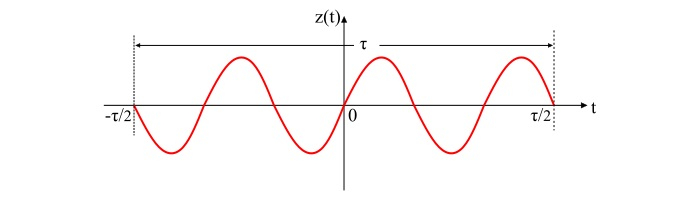
The signal $\mathrm{Z(t)}$ is given by,

$$\mathrm{Z\left(t\right)=\begin{cases} x(t)\:\left|t \right|\lt\left ( \frac{\tau }{2} \right )\\\\ 0 \: {otherwise } \end{cases}}$$

Where,$\mathrm{x(t)}$ is a power signal of same magnitude extending to infinity.

As the signal $\mathrm{Z(t)}$ is finite duration signal of duration $\tau$ and thus, it is an energy signal having energy E, that is given by,

$$\mathrm{E\:=\:\int_{-\infty}^{\infty}\left|Z(t)\right|^{2}\:dt\:=\:\frac{1}{2\pi}\int_{-\infty}^{\infty}\left| Z(\omega) \right|^{2}\:d\omega}$$

Where,

$$\mathrm{Z(t)\overset{FT}{\leftrightarrow}Z(\omega)}$$

Also,

$$\mathrm{\int_{-\infty}^{\infty}\left|Z(t)\right|^{2}\:dt\:=\:\int_{-(\tau/2)}^{(\tau/2)}\left| x(t)\right|^{2}\:dt}$$

Therefore, we have,

$$\mathrm{\frac{1}{\tau}\int_{-(\tau/2)}^{(\tau /2)}\left| x(t)\right|^{2}\:dt\:=\:\frac{1}{2\pi}\left(\frac{1} {\tau}\right)\int_{-\infty}^{\infty}\left| Z(\omega)\right|^{2}\:d\omega}$$

Hence, when $\mathrm{\tau \:\to\: \infty}$, then the LHS of the above equation gives the average power (P) of the signal $x\mathrm{(t)}$ , i.e.,

$$\mathrm{P\:=\:\frac{1}{2\pi}\int_{-\infty}^{\infty}\displaystyle \lim_{\tau \:\to\:\infty}\left(\frac{\left| Z(\omega) \right|^{2}}{\tau}\right)\:d\omega\:\: ... \:(2)}$$

If $\mathrm{\tau\:\to\:\infty}$, then $\mathrm{\left(\frac{\left| Z(\omega)\right|^{2}}{\tau}\right)}$ in equation (2) approaches a finite value. Assume this finite value is represented by $\mathrm{S(\omega)}$, i.e.,

$$\mathrm{S(\omega)\:=\:\displaystyle \lim_{\tau \:\to\:\infty}\left(\frac{\left| Z(\omega)\right|^{2}}{\tau}\right) \:\: ...\:(3)}$$

The expression in the equation (3) is called the power spectral density (PSD) of the signal $\mathrm{z(t)}$. Therefore, for the function $x\mathrm{\left(\mathrm{t}\right)}$, the PSD function is given by,

$$\mathrm{S\left(\omega\right)\:=\:\displaystyle \lim_{\tau \:\to\:\infty}\left(\frac{\left| X(\omega)\right|^{2}}{\tau} \right) \:\: ...\:(4)}$$

Hence, the average power (P) of the signal $\mathrm{x(t)}$ is given by,

$$\mathrm{P\:=\:\frac{1}{2\pi}\int_{-\infty}^{\infty}S(\omega)\:d\omega \:=\:\int_{-\infty}^{\infty}S(f) \: df\:\: ...\:(5)}$$

Also, the power spectral density (PSD) of a periodic function is given by,

$$\mathrm{S(\omega)\:=\:2\pi\:\sum_{n=-\infty}^{\infty}\left|c_{n}\right|^{2}\delta(\omega\:-\:n\omega_{0})}\:\:...\:(6)$$

Properties of Power Spectral Density (PSD)

Property 1 - For a power signal, the area under the power spectral density curve is equal to the average power of that signal, i.e.,

$$\mathrm{P\:=\:\frac{1}{2\pi}\int_{-\infty}^{\infty}\:S(\omega)\:d\omega}$$

Property 2 - If the signal $\mathrm{x(t)}$ is input to an LTI system with impulse response $\mathrm{h(t)}$, then the input and output PSD functions of the system are related as,

$$\mathrm{S_{y}(\omega)\:=\:\left|H(\omega)\right|^{2}\:S_{x}(\omega)}$$

Where,$\mathrm{\left|H(\omega)\right|}$ is the magnitude of the system transfer function.

Property 3 - The autocorrelation function $\mathrm{R(\tau)}$ and the power spectral density function $\mathrm{S(\omega)}$ of a power signal form a Fourier transform pair, i.e.,

$$\mathrm{R(\tau)\:\overset{FT}\:{\leftrightarrow}\:S(\omega)}$$