Transform Analysis of LTI Systems using Z-Transform

---

---

Z-Transform

The Z-transform is a mathematical tool which is used to convert the difference equations in discrete time domain into the algebraic equations in z-domain. Mathematically, if x(n) is a discrete time function, then its Z-transform is defined as,

$$\mathrm{Z\left[x(n)\right]\:=\:X(z)\:=\: \sum_{n=-\infty}^{\infty}\: x(n) z^{-n}}$$

Transform Analysis of Discrete-Time System

The Z-transform plays a vital role in the design and analysis of discrete-time LTI (Linear Time Invariant) systems.

Transfer Function of a Discrete-Time LTI System

The figure shows a discrete-time LTI system having an impulse response h(n).

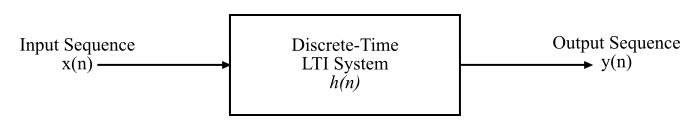
Consider the system gives an output y(n) for an input x(n). Then,

$$\mathrm{y(n) \:=\: h(n) \:\cdot\: x(n)}$$

Taking Z-transform on both the sides, we get,

$$\mathrm{Z\left[y(n)\right] \:=\: Z\left[h(n) \:\cdot\: x(n)\right]}$$

$$\mathrm{\therefore\: Y(z)\:=\:H(z)X(z)}$$

Therefore, the Z-transform of the impulse response h(n) of the system is given by,

$$\mathrm{H(z) \:=\: \frac{Y(z)}{X(z)}}$$

Where, H(z) is called the transfer function of the discrete-time LTI system and can be defined as follows −

The transfer function of a discrete time LTI system is defined as the ratio of Z-transform of the output sequence to the Z-transform of the input sequence x(n), when the initial conditions are neglected.

Relationship between Transfer Function and Difference Equation of Discrete Time LTI System

An n^th order discrete-time LTI system is described in terms of a difference equation as follows −

$$\mathrm{\sum_{k=0}^{N}\: a_k y(n\:-\:k) \:=\: \sum_{k=0}^{M}\: b_k x(n\:-\:k)}$$

On expanding the above difference equation, we get,

$$\mathrm{a_0 y(n) \:+\: a_1 y(n\:-\:1) \:+\: a_2 y(n\:-\:2) \:+\: a_3 y(n\:-\:3) \:+\:\dots \:+\: a_N y(n\:-\:N) \:=\: b_0 x(n) \:+\: b_1 x(n\:-\:1) \:+\: b_2 x(n\:-\:2) \:+\:b_3 x(n\:-\:3) \:+\: \dots \:+\: b_M x(n\:-\:M)}$$

Taking Z-transform on both sides and neglecting the initial conditions, we get,

$$\mathrm{Z\left[a_0 y(n) \:+\: a_1 y(n\:-\:1) \:+\: a_2 y(n\:-\:2) \:+\: a_3 y(n\:-\:3) \:+\: \dots \:+\: a_N y(n\:-\:N)\right] \:=\: Z\left[b_0 x(n) \:+\: b_1 x(n\:-\:1) \:+\: b_2 x(n\:-\:2) \:+\: b_3 x(n\:-\:3) \:+\: \dots \:+\: b_M x(n\:-\:M)\right]}$$

$$\mathrm{\Rightarrow\: a_0 Y(z) \:+\: a_1 z^{-1} Y(z) \:+\: a_2 z^{-2} Y(z) \:+\: a_3 z^{-3} Y(z) \:+\: \dots \:+\: a_N z^{-N} Y(z) \:=\:b_0 X(z) \:+\:b_1 z^{-1} X(z) \:+\: b_2 z^{-2} X(z) \:+ \:b_3 z^{-3} X(z) \:+\: \dots \:+\: b_M z^{-M} X(z)}$$

$$\mathrm{\Rightarrow\: \left[a_0 \:+\: a_1 z^{-1} \:+\: a_2 z^{-2} \:+\: a_3 z^{-3} \:+\: \dots \:+\: a_N z^{-N}\right] Y(z) \:=\: \left[b_0 \:+\: b_1 z^{-1} \:+\: b_2 z^{-2} \:+\: b_3 z^{-3} \:+\: \dots \:+\: b_M z^{-M}\right]\: X(z)}$$

$$\mathrm{\Rightarrow\: \frac{Y(z)}{X(z)} \:=\: \frac{b_0 \:+\: b_1 z^{-1} \:+\: b_2 z^{-2} \:+\: b_3 z^{-3} \:+\: \dots \:+\: b_M z^{-M}}{a_0 \:+\: a_1 z^{-1} \:+\: a_2 z^{-2} \:+\: a_3 z^{-3} \:+\: \dots \:+\: a_N z^{-N}}}$$

$$\mathrm{\therefore\: \frac{Y(z)}{X(z)} \:=\: H(z) \:=\: \frac{\sum_{k=0}^{M}\: b_k z^{-k}}{\sum_{k=0}^{N} a_k z^{-k}}}$$

Where, H(z) is the transfer function of the discrete-time system and the above equation gives the relation between the transfer function and the difference equation of the system.