Signals Sampling Techniques

---

---

There are three types of sampling techniques:

• Impulse sampling.

• Natural sampling.

• Flat Top sampling.

Impulse Sampling

Impulse sampling can be performed by multiplying input signal x(t) with impulse train $\Sigma_{n=-\infty}^{\infty}\delta(t-nT)$ of period 'T'. Here, the amplitude of impulse changes with respect to amplitude of input signal x(t). The output of sampler is given by

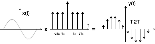
$y(t) = x(t) $ impulse train

$= x(t) \Sigma_{n=-\infty}^{\infty} \delta(t-nT)$

$ y(t) = y_{\delta} (t) = \Sigma_{n=-\infty}^{\infty}x(nt) \delta(t-nT)\,...\,... 1 $

To get the spectrum of sampled signal, consider Fourier transform of equation 1 on both sides

$Y(\omega) = {1 \over T} \Sigma_{n=-\infty}^{\infty} X(\omega - n \omega_s ) $

This is called ideal sampling or impulse sampling. You cannot use this practically because pulse width cannot be zero and the generation of impulse train is not possible practically.

Natural Sampling

Natural sampling is similar to impulse sampling, except the impulse train is replaced by pulse train of period T. i.e. you multiply input signal x(t) to pulse train $\Sigma_{n=-\infty}^{\infty} P(t-nT)$ as shown below

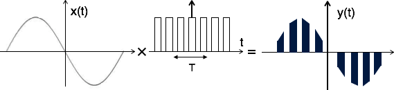
The output of sampler is

$y(t) = x(t) \times \text{pulse train}$

$= x(t) \times p(t) $

$= x(t) \times \Sigma_{n=-\infty}^{\infty} P(t-nT)\,...\,...(1) $

The exponential Fourier series representation of p(t) can be given as

$p(t) = \Sigma_{n=-\infty}^{\infty} F_n e^{j n\omega_s t}\,...\,...(2) $

$= \Sigma_{n=-\infty}^{\infty} F_n e^{j 2 \pi nf_s t} $

Where $F_n= {1 \over T} \int_{-T \over 2}^{T \over 2} p(t) e^{-j n \omega_s t} dt$

$= {1 \over TP}(n \omega_s)$

Substitute F_n value in equation 2

$ \therefore p(t) = \Sigma_{n=-\infty}^{\infty} {1 \over T} P(n \omega_s)e^{j n \omega_s t}$

$ = {1 \over T} \Sigma_{n=-\infty}^{\infty} P(n \omega_s)e^{j n \omega_s t}$

Substitute p(t) in equation 1

$y(t) = x(t) \times p(t)$

$= x(t) \times {1 \over T} \Sigma_{n=-\infty}^{\infty} P(n \omega_s)\,e^{j n \omega_s t} $

$y(t) = {1 \over T} \Sigma_{n=-\infty}^{\infty} P( n \omega_s)\, x(t)\, e^{j n \omega_s t} $

To get the spectrum of sampled signal, consider the Fourier transform on both sides.

$F.T\, [ y(t)] = F.T [{1 \over T} \Sigma_{n=-\infty}^{\infty} P( n \omega_s)\, x(t)\, e^{j n \omega_s t}]$

$ = {1 \over T} \Sigma_{n=-\infty}^{\infty} P( n \omega_s)\,F.T\,[ x(t)\, e^{j n \omega_s t} ] $

According to frequency shifting property

$F.T\,[ x(t)\, e^{j n \omega_s t} ] = X[\omega-n\omega_s] $

$ \therefore\, Y[\omega] = {1 \over T} \Sigma_{n=-\infty}^{\infty} P( n \omega_s)\,X[\omega-n\omega_s] $

Flat Top Sampling

During transmission, noise is introduced at top of the transmission pulse which can be easily removed if the pulse is in the form of flat top. Here, the top of the samples are flat i.e. they have constant amplitude. Hence, it is called as flat top sampling or practical sampling. Flat top sampling makes use of sample and hold circuit.

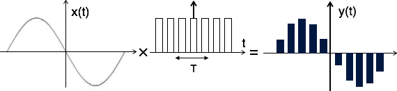
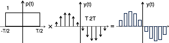
Theoretically, the sampled signal can be obtained by convolution of rectangular pulse p(t) with ideally sampled signal say y_δ(t) as shown in the diagram:

i.e. $ y(t) = p(t) \times y_\delta (t)\, ... \, ...(1) $

To get the sampled spectrum, consider Fourier transform on both sides for equation 1

$Y[\omega] = F.T\,[P(t) \times y_\delta (t)] $

By the knowledge of convolution property,

$Y[\omega] = P(\omega)\, Y_\delta (\omega)$

Here $P(\omega) = T Sa({\omega T \over 2}) = 2 \sin \omega T/ \omega$

Nyquist Rate

It is the minimum sampling rate at which signal can be converted into samples and can be recovered back without distortion.

Nyquist rate f_N = 2f_m hz

Nyquist interval = ${1 \over fN}$ = $ {1 \over 2fm}$ seconds.

Samplings of Band Pass Signals

In case of band pass signals, the spectrum of band pass signal X[ω] = 0 for the frequencies outside the range f₁ ≤ f ≤ f₂. The frequency f₁ is always greater than zero. Plus, there is no aliasing effect when f_s > 2f₂. But it has two disadvantages:

• The sampling rate is large in proportion with f₂. This has practical limitations.

• The sampled signal spectrum has spectral gaps.

To overcome this, the band pass theorem states that the input signal x(t) can be converted into its samples and can be recovered back without distortion when sampling frequency f_s < 2f₂.

Also,

$$ f_s = {1 \over T} = {2f_2 \over m} $$

Where m is the largest integer < ${f_2 \over B}$

and B is the bandwidth of the signal. If f₂=KB, then

$$ f_s = {1 \over T} = {2KB \over m} $$

For band pass signals of bandwidth 2f_m and the minimum sampling rate f_s= 2 B = 4f_m,

the spectrum of sampled signal is given by $Y[\omega] = {1 \over T} \Sigma_{n=-\infty}^{\infty}\,X[ \omega - 2nB]$