Systems Classification

---

---

Systems are classified into the following categories:

• linear and Non-linear Systems
• Time Variant and Time Invariant Systems
• linear Time variant and linear Time invariant systems
• Static and Dynamic Systems
• Causal and Non-causal Systems
• Invertible and Non-Invertible Systems
• Stable and Unstable Systems

linear and Non-linear Systems

A system is said to be linear when it satisfies superposition and homogenate principles. Consider two systems with inputs as x₁(t), x₂(t), and outputs as y₁(t), y₂(t) respectively. Then, according to the superposition and homogenate principles,

T [a₁ x₁(t) + a₂ x₂(t)] = a₁ T[x₁(t)] + a₂ T[x₂(t)]

$\therefore, $ T [a₁ x₁(t) + a₂ x₂(t)] = a₁ y₁(t) + a₂ y₂(t)

From the above expression, is clear that response of overall system is equal to response of individual system.

Example:

(t) = x²(t)

Solution:

y₁ (t) = T[x₁(t)] = x₁²(t)

y₂ (t) = T[x₂(t)] = x₂²(t)

T [a₁ x₁(t) + a₂ x₂(t)] = [ a₁ x₁(t) + a₂ x₂(t)]²

Which is not equal to a₁ y₁(t) + a₂ y₂(t). Hence the system is said to be non linear.

Time Variant and Time Invariant Systems

A system is said to be time variant if its input and output characteristics vary with time. Otherwise, the system is considered as time invariant.

The condition for time invariant system is:

y (n , t) = y(n-t)

The condition for time variant system is:

y (n , t) $\neq$ y(n-t)

Where y (n , t) = T[x(n-t)] = input change

y (n-t) = output change

Example:

y(n) = x(-n)

y(n, t) = T[x(n-t)] = x(-n-t)

y(n-t) = x(-(n-t)) = x(-n + t)

$\therefore$ y(n, t) y(n-t). Hence, the system is time variant.

linear Time variant (LTV) and linear Time Invariant (LTI) Systems

If a system is both linear and time variant, then it is called linear time variant (LTV) system.

If a system is both linear and time Invariant then that system is called linear time invariant (LTI) system.

Static and Dynamic Systems

Static system is memory-less whereas dynamic system is a memory system.

Example 1: y(t) = 2 x(t)

For present value t=0, the system output is y(0) = 2x(0). Here, the output is only dependent upon present input. Hence the system is memory less or static.

Example 2: y(t) = 2 x(t) + 3 x(t-3)

For present value t=0, the system output is y(0) = 2x(0) + 3x(-3).

Here x(-3) is past value for the present input for which the system requires memory to get this output. Hence, the system is a dynamic system.

Causal and Non-Causal Systems

A system is said to be causal if its output depends upon present and past inputs, and does not depend upon future input.

For non causal system, the output depends upon future inputs also.

Example 1: y(n) = 2 x(t) + 3 x(t-3)

For present value t=1, the system output is y(1) = 2x(1) + 3x(-2).

Here, the system output only depends upon present and past inputs. Hence, the system is causal.

Example 2: y(n) = 2 x(t) + 3 x(t-3) + 6x(t + 3)

For present value t=1, the system output is y(1) = 2x(1) + 3x(-2) + 6x(4) Here, the system output depends upon future input. Hence the system is non-causal system.

Invertible and Non-Invertible systems

A system is said to invertible if the input of the system appears at the output.

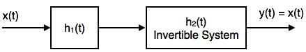
Y(S) = X(S) H1(S) H2(S)

= X(S) H1(S) $1 \over ( H1(S) )$       Since H2(S) = 1/( H1(S) )

$\therefore, $ Y(S) = X(S)

$\to$ y(t) = x(t)

Hence, the system is invertible.

If y(t) $\neq$ x(t), then the system is said to be non-invertible.

Stable and Unstable Systems

The system is said to be stable only when the output is bounded for bounded input. For a bounded input, if the output is unbounded in the system then it is said to be unstable.

Note: For a bounded signal, amplitude is finite.

Example 1: y (t) = x²(t)

Let the input is u(t) (unit step bounded input) then the output y(t) = u2(t) = u(t) = bounded output.

Hence, the system is stable.

Example 2: y (t) = $\int x(t)\, dt$

Let the input is u (t) (unit step bounded input) then the output y(t) = $\int u(t)\, dt$ = ramp signal (unbounded because amplitude of ramp is not finite it goes to infinite when t $\to$ infinite).

Hence, the system is unstable.